Plugin not installed

Step-by-Step Monte Carlo Simulation in Python for Trading and Portfolio Risk Analysis

Author

Abe Cofnas

Last update: 10 February 2026

Reading time: 23 min

Monte Carlo Simulation in Python is a practical way to turn trading uncertainty into numbers you can plan around.

This guide shows how to structure a simulation workflow that is repeatable, transparent, and easy to audit. You will learn which inputs matter most, which outputs deserve your attention, and how to turn results into clear risk limits and portfolio choices.

Trading involves risk of loss, and simulations do not remove that risk; they help you measure it under stated assumptions.

Key Points:

Monte Carlo Simulation in Python turns a single backtest into a probability map of drawdowns, not a single “true” outcome.

Small changes in trade order can produce large equity differences, so sequence risk is often bigger than signal quality.

Portfolio Monte Carlo is most useful when you compare allocations by Sharpe stability and worst-case drawdown, not by peak returns.
Reproducible results require fixed inputs, saved seeds, and versioned data, or your “improvements” may be random noise.

Understanding Monte Carlo Simulation in Trading

In this section, you will learn what a Monte Carlo simulation is and why traders use it. We also outline its main applications in portfolio risk, option pricing, and strategy stress-testing.

What Monte Carlo Simulation Means for Trading and Risk Analysis

Monte Carlo simulation is a method for modelling market uncertainty. You run the same model multiple times, and in each run, you randomly change the inputs according to a defined rule or probability distribution.

Instead of one single result, you get a distribution of outcomes. This distribution shows the possible outcomes across different scenarios.

Key Point
For a trader, the Monte Carlo output is usually not one fixed number like “expected return”. The key output is a range of results that shows how best-case, typical, and worst-case outcomes may look. This helps you see real risk, not only the average.

Key Financial Applications: Portfolio, Options, and Strategy Stress-Testing

1) Portfolio (investment basket):

Monte Carlo helps you estimate the probability of reaching a specific loss level. This estimate is usually based on assumptions such as expected returns, volatility, and asset correlations. In simple terms, you can answer: “With this portfolio mix, what is the chance I lose 10% within a given time period?”

2) Derivatives and options:

For option pricing, Monte Carlo is very useful when a closed-form formula does not exist or when applying it to complex setups is difficult. It is also common when the option payoff is path-dependent, meaning the payoff depends on the price path, not just the final price.

Trading Strategy Stress-Testing

A backtest shows one historical sequence of wins and losses, but live trading can deliver the same trades in a different order. Monte Carlo stress testing reshuffles or resamples returns to generate many alternative equity curve paths.

This shows how sensitive your results are to losing streaks, volatility shifts, and adverse sequences. The goal is to check whether the strategy remains acceptable across many scenarios, not just in a single favourable backtest period.

Why Backtests Look Cleaner Than Live Trading

Backtests can look smooth because they reflect one specific historical order of outcomes. Even with the same win rate and average trade, a different sequence can create deeper drawdowns and longer recovery periods.

Imagine two traders start with $10,000 and both earn 10% total return after 4 trades.

Trader A (Steady): +2.5%, +2.5%, +2.5%, +2.5%. Result: Smooth growth.

Trader B (Volatile): -50%, +50%, -20%, +65%. Result: Deep drawdown and stress.

The Lesson: A simple backtest sees only the end result ($11,000). Monte Carlo reveals the path (Trader B likely quit during the -50% drop).

This is called sequence risk:
The order of returns can change risk, even when average performance looks similar.

Quick-Start: Monte Carlo Simulation in Python for Trading

In this section, you will build a basic Monte Carlo workflow in Python, from sampling returns to generating equity curve paths. You will also learn how to export results and read key risk outputs such as drawdown percentiles and VaR.

Step-by-Step Guide to Running Monte Carlo Simulations

According to Investopedia, to run a Monte Carlo simulation for a trading strategy, follow a clear and repeatable process.

Step 1: Prepare your inputs.
Collect your strategy’s return series, such as daily returns or per-trade returns. Include fees and slippage if possible, because they change real results.

Step 2: Choose a simulation method.
Use bootstrap resampling to reshuffle or resample historical returns. Or use parametric sampling to assume a distribution and generate random returns.

Step 3: Run many simulation paths.
Repeat the process thousands of times. In each run, compound returns to build an equity curve for that path.

Step 4: Summarise and interpret risk.
Analyse the distributions of ending equity, maximum drawdown, and worst-case percentiles. Add the Sharpe ratio and confidence ranges to measure risk and uncertainty.

Python Code Example: Simulating Equity Curve Paths

Use NumPy’s modern random generator for repeatable sampling, then compound returns into an equity curve for each simulation path.

import numpy as np

rng = np.random.default_rng(42)

returns = np.array([0.002, -0.001, 0.0005, 0.003, -0.002]) # example daily returns

n_paths = 5000

horizon = 252

sim = rng.choice(returns, size=(n_paths, horizon), replace=True)

equity = (1.0 + sim).cumprod(axis=1)

ending_equity = equity[:, -1]

Exporting Results and Visualising Strategy Outcomes

To make your simulation results easier to compare, save the final equity and drawdown for each path in a table. This lets you compare different strategy settings or parameter sets using the same reporting format.

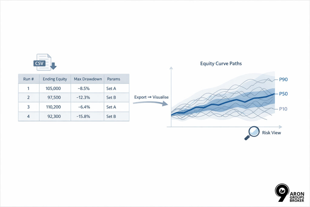
Next, plot several random equity curve paths and add percentile bands such as P10, P50, and P90. This view helps you understand risk faster, because ranges show uncertainty better than a single average.

Calculating Max Drawdown in Python

Maximum drawdown measures the worst peak-to-trough decline in an equity curve, expressed as a percentage from the prior peak.

In a Monte Carlo test, compute max drawdown for each simulated equity path and store the result as one value per path. This gives you an array of drawdowns that you can analyse later with percentiles and risk limits.

def max_drawdown(equity_curve: np.ndarray) -> float:

peak = np.maximum.accumulate(equity_curve)

dd = (equity_curve / peak) – 1.0

return float(dd.min())

mdd = np.apply_along_axis(max_drawdown, 1, equity)

Understanding Key Risk Metrics: Sharpe Ratio and Confidence Intervals

The Sharpe ratio measures risk-adjusted performance by comparing average excess return to return volatility. A higher Sharpe usually means smoother returns for the same level of return.

To compute Sharpe: you estimate average return, subtract a risk-free rate (if used), then divide by the standard deviation of returns over the same period.

Confidence intervals describe uncertainty around an estimate. They show a likely range for a metric, such as Sharpe or drawdown, at a chosen confidence level.

Core Risk Metrics for Traders

In this section, you will learn how to read three core Monte Carlo risk outputs, so you can set clearer risk limits.

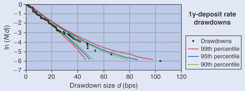
Maximum Drawdown Distribution Across Simulations

A drawdown distribution answers a practical trading question: how often does this strategy breach my loss tolerance?

Focus on percentile levels, especially P90 to P99, because these outcomes often drive margin stress, forced exits, and poor decision-making under pressure. Use the distribution to set limits, such as “P95 drawdown must stay below X%”, rather than relying on one historical drawdown number.

Risk Limit Checklist: Is My Strategy Broken? Run your simulation and check these 3 "Pain Points":

P50 (Median): Is the typical drawdown acceptable? (e.g., < 15%).

P95 (Worst Case): Can my account survive the 95th percentile loss? (e.g., < 30%).

Bankruptcy Risk: What percentage of paths hit -100% or my liquidation level? (Must be 0%).

Value at Risk (VaR) Using Monte Carlo Simulation

Value at Risk (VaR) estimates a loss level that should not be exceeded at a chosen confidence level over a defined time horizon.

For example, a 95% one-day VaR estimates a loss level that should not be breached on most trading days.

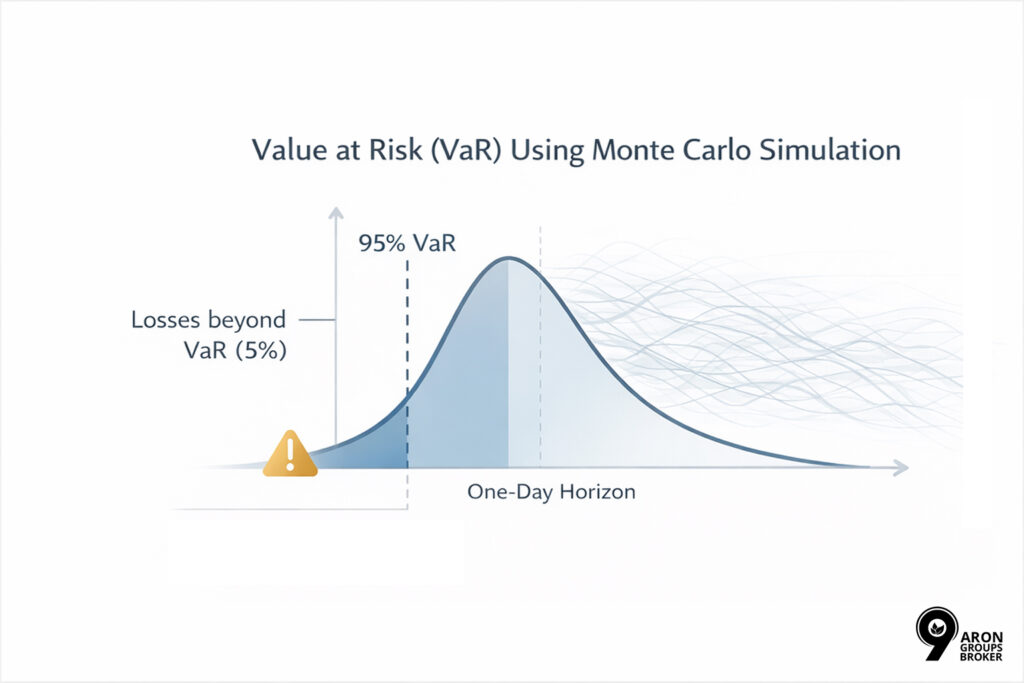
Monte Carlo VaR is flexible, but it depends on the model and its assumptions. If your assumptions are weak or unrealistic, VaR can understate true risk and create false confidence.

Tail Risk and Slippage Analysis

Tail risk is the chance of rare but very large losses. For leveraged traders, tail events often matter more than average volatility. Include slippage and wider spreads in your simulations, because execution costs rise when liquidity is thin and price moves quickly.

This helps you measure how much performance can change when fills are worse than your backtest assumptions.

Applying Monte Carlo to Portfolio and Strategy Optimisation

In this section, you use Monte Carlo outputs to compare portfolio allocations. The focus is on weight constraints, diversification behaviour under changing correlations, and portfolio selection using the efficient frontier and Sharpe-based trade-offs.

Portfolio Risk and Diversification Considerations

Diversification works best when assets have low, stable correlations. However, correlation is not constant. During market stress, correlations often rise towards one, and many assets can fall together.

Monte Carlo allows you to test this behaviour measurably by running portfolio simulations under different regimes, such as:

Calm market conditions: lower volatility and lower correlation.
Stressed market conditions: higher volatility and higher correlation.

By simulating both regimes, you can see whether diversification helps only in normal markets or whether it also reduces risk in the worst periods. This is critical for managing large equity drawdowns because major losses often occur during stressed conditions.

Random Weight Allocation Techniques

With random weight allocation, you generate thousands of portfolio weight sets instead of testing only one or two “guessed” allocations.

For example, in a four-asset portfolio, you create four weights that sum to 100%, then evaluate risk and return for each set.

Random does not mean unrealistic. You should add practical constraints, such as:

A maximum weight per asset (for example, no asset above 30%).
No leverage or short selling, if you do not trade that way in practice.
Minimum weights for core holdings, if your portfolio must keep a defined structure.

These constraints make the output tradable and relevant, not only a mathematical exercise.

Portfolio Optimisation Python Code Workflow

A practical and repeatable workflow usually follows these steps:

Define inputs: historical returns, volatilities, and a correlation or covariance matrix.
Generate weights: create many weight sets while applying your constraints.
Compute portfolio returns: build the combined return series from the weights.
Run Monte Carlo: simulate many performance paths for each weight set.
Store outputs: ending equity, max drawdown, VaR, and Sharpe ratio.
Rank results: use a clear objective, such as the lowest P95 drawdown or the most stable Sharpe.

The key point is consistency. If you want to compare several allocations, keep your assumptions unchanged. If you change sampling rules, cost inputs, or time horizon mid-test, the comparison becomes unreliable.

Selecting Portfolios by Sharpe Stability

A common mistake is choosing a portfolio based on the highest Sharpe ratio in a single backtest. This can reflect noise or a favourable period rather than a durable allocation.

Use Monte Carlo outputs to judge Sharpe stability across many simulated paths. Review the median Sharpe, how Sharpe behaves in low percentile ranges such as P10, and how often Sharpe turns negative.

A portfolio with a slightly lower average Sharpe but stable outcomes across paths is often more usable in real trading than a portfolio with one very high Sharpe in one sample.

Efficient Frontier Visualisation

The efficient frontier is the set of portfolios that deliver the highest expected return for a given level of risk.
In simple terms, each point on the frontier says: “If you accept this risk level, this is the best return you can target.”

In practice, you typically:

Plot all simulated portfolios on a risk-return chart.
Identify the best points that form the efficient frontier.
Highlight the region near the highest Sharpe ratio, as it offers a stronger return-to-risk trade-off.

However, Sharpe alone is not enough for real decisions. You should also review:

Drawdown levels in the worst percentiles.
The probability of severe losses, including VaR.
Whether the portfolio remains tolerable under stressed regimes.

The efficient frontier is a decision tool, not a profit guarantee, because all results depend on assumptions and future market behaviour.

Monte Carlo Option Pricing and Stock Price Modelling

In this section, the goal is to understand how Monte Carlo builds many possible price paths. This helps you view future stock prices in probabilities and estimate a fair option value by averaging payoffs across many scenarios.

Geometric Brownian Motion Explained

Geometric Brownian Motion (GBM) is one of the most common simple models for simulating stock prices. It has two main ideas:

Returns are random.
Each time step (for example, each day) includes an expected component and a random shock.
Volatility scales with the price level.
When the price is higher, the absolute price movement is often larger, because volatility is treated as a percentage.

In practice, GBM often assumes that log returns are approximately normal and that volatility remains constant throughout the simulation.

This is a simplification, and it can fail in real markets, especially:

During price jumps;
During sharp sell-offs or crashes;
When volatility shifts between regimes (calm periods and stressed periods).

Note:
Even with these limits, GBM is useful for learning Monte Carlo mechanics because the model is clear and easy to implement.

Simulating Future Stock Prices in Python

When you simulate GBM paths in Python, you do not produce one “precise” forecast line. Instead, you generate many price paths, each representing a possible future scenario.

The main output is:

A set of simulated paths, and
A distribution of future prices at a chosen date (for example, day 30 or day 252)

This approach is practical because it supports probability questions. For example:

What is the probability that the price ends the month below 100?
What is the probability that the price moves above 130?

For risk management, these probabilities are often more useful than a single-point estimate, because markets are inherently uncertain.

Monte Carlo Option Pricing Principles and Python Code

In Monte Carlo option pricing, the logic is straightforward:

Simulate the underlying price paths
For example, generate thousands of stock price paths up to the option expiry.
Calculate the option payoff for each path
For a call option at expiry: If the final price is above the strike, the payoff is positive. If it is below, the payoff is zero.
Take the average payoff across all paths
Each path represents one scenario, so the average gives an estimate of the expected payoff.
Discount the average payoff back to today
You apply a suitable discount rate to convert the expected payoff into a present value, which becomes the option price today.

The main advantage of Monte Carlo is that it can handle complex payoffs that are difficult to price with simple formulas.

It is especially useful when:

The payoff is path-dependent, not only based on the final price.
The option has custom features.
You want to include practical assumptions, such as execution or modelling constraints.

Comparing Monte Carlo Pricing with Black-Scholes

Black-Scholes is a closed-form model for pricing certain standard options. Its key points are:

It is very fast when its assumptions fit the contract.
The method is transparent because the formula is explicit.
It relies on strict assumptions, such as constant volatility and no sudden jumps.

Monte Carlo is usually:

Slower, because it runs many simulations,
But more flexible for complex or customised payoffs.

Q: When should traders use Black-Scholes instead of Monte Carlo for option pricing?
A: So, there is no single “best” method in every case. For simple, standard options, Black-Scholes is often sufficient and efficient. For complex contracts or custom features, Monte Carlo is often the more suitable choice.

Monte Carlo for Time Series Forecasting

In this section, you will apply Monte Carlo to financial time series using resampling methods such as the bootstrap. You will also see how to combine simulations with forecasting models by simulating forecast errors and uncertainty bands.

Resampling Techniques for Financial Time Series

Bootstrap resampling builds synthetic paths by reordering historical returns, thereby preserving features such as skew, fat tails, and volatility clustering. Because markets change, test several lookback windows, such as one, three, and five years, and compare the outputs.

When volatility varies across periods, run separate simulations for each regime window rather than using a single blended sample.

Forecasting Price Paths Under Uncertainty

Simulated paths are useful because they help you plan risk before you place a trade.
For example, you can use the paths to make these decisions more measurable:

Stop distance: estimate the share of paths where normal volatility would hit the stop.
Position size: size the trade based on adverse scenarios, so drawdown stays within limits.
Loss sequence tolerance: test how your equity reacts if several losses occur in a row.

Important:
The key point is that Monte Carlo paths are not guaranteed predictions. They show a conditional range of outcomes: “If your data and assumptions are reasonable, these results are possible.” So, output quality depends on data quality, cost assumptions, and the chosen sampling method.

Integrating Simulations with Predictive Models

Sometimes you use a forecasting model, such as a statistical or machine learning model, to estimate direction or returns. A common mistake is to simulate only the model’s forecast and ignore forecast error.

For a more realistic view, you should also simulate forecast errors, because:

Models often miss turning points in real time.
Real markets show fat tails and unusual moves that models often underestimate.

This integration is most valuable when it changes your decisions. For example, if uncertainty bands widen meaningfully, you may:

Reduce position size,
Set a more realistic stop loss, or
Stay out of the trade until conditions become clearer.

So, the goal is not “price prediction”. The goal is to develop a practical decision framework for decision-making under uncertainty.

Python Libraries and Technical Foundations for Monte Carlo Simulation

In this section, you will learn the core Python tools and technical points that determine Monte Carlo quality.

Essential Python Libraries: NumPy, Pandas, Matplotlib

NumPy is the primary library for numerical computing in Python. In Monte Carlo, it is used to:

Build and manage large arrays (for example, thousands of paths over 252 trading days).
Generate random samples and pseudo-random numbers.
Run vectorised calculations that are much faster than standard Python loops.

Pandas is primarily for data management, not the simulation core. It helps you:

Store results for each path or scenario in a clean table (DataFrame).
Filter outputs (for example, isolate the worst 5% outcomes).
Export reports to CSV or Excel to compare different parameter settings.

Matplotlib makes risk visible. It is commonly used to plot:

Distributions of ending equity or drawdowns (histograms).
A sample of equity curve paths.
Percentile bands (P10, P50, P90) to show plausible outcome ranges. This reduces the risk of hiding uncertainty inside a few summary statistics.

Advanced Libraries for Monte Carlo Simulation

When the number of paths, assets, or scenarios grows, simulations can become slow.
At that stage, you can use optimisation and parallel tools, such as:

Numba to speed up heavy numerical functions.
joblib or built-in tools like multiprocessing and concurrent.futures to run tasks across CPU cores.
Dask or Ray for much larger workloads and more scalable execution.

However, the priority is always: validate the simulation logic first, then improve speed. If the model is wrong, faster runs only produce wrong outputs more quickly.

These libraries are most useful when:

Inputs are stable and clearly defined.
You have basic checks (for example, mean and volatility behave as expected).
Results are consistent across repeated runs and do not show unusual instability.

Probability Distributions and Random Sampling Techniques

The most important Monte Carlo choice is how you generate returns. Your sampling method shapes your results, so choose it deliberately. Common options include:

Normal draws: simple and fast, but may understate heavy tails.
t-distribution draws: better when you want larger moves to appear more realistically.
Bootstrap resampling: sample from observed returns without assuming normality.

If your strategy has skewed outcomes, a normal assumption can understate tail losses. This risk is higher with leverage or options exposure.

Normal Distribution, Standard Deviation, and Confidence Intervals

Standard deviation measures dispersion, but it treats upside and downside volatility equally. This can be misleading for traders who care most about drawdowns and downside risk.

Confidence intervals add context by reporting a range rather than one exact value.

For example, instead of saying “average drawdown is 12%”, you can say: “With 90% probability, drawdown falls between 8% and 20%.”

This is usually safer for risk decisions than a single “best estimate”.

Iterations, Convergence, and Simulation Stability

More iterations usually reduce sampling noise. However, more runs do not fix weak assumptions. If your return or cost model is wrong, even one million paths will not make the results valid.

To check stability, two practical steps are:

Repeat runs with different random seeds and measure how much the results change.
Increase iterations and track key percentiles (such as P5 or P10 drawdown).
If these percentiles still move materially, your simulation has not stabilised yet.

This approach helps ensure Monte Carlo results are technically sound, not only attractive numbers.

Applying Monte Carlo to Quantitative Trading Strategies

Strategy Validation and Robustness Testing

A backtest usually shows only one historical path, with one specific sequence of wins and losses.
In live trading, the same win rate and average profit can produce very different equity curves when the sequence changes.

Monte Carlo tests this directly by:

Reordering trade outcomes many times or resampling historical returns.
Building thousands of new equity curve paths.
Measuring whether the strategy remains acceptable across many scenarios.

Example: Suppose your strategy has 200 trades, a 55% win rate, and an average trade result of +0.15R. In the backtest, the worst losing streak was seven trades.

After Monte Carlo, you may find:

In 50% of paths, the worst losing streak is six to nine trades.
In 10% of paths, the losing streak reaches 13 trades.
In 5% of paths, the maximum drawdown exceeds 20%.

This creates a practical question: Can you tolerate 13 losses in a row, or would you stop trading the system mid-cycle?

Position Sizing and Capital Allocation Simulations

Many traders focus on entry signals, but position sizing often determines whether drawdowns become dangerous. For this reason, you should simulate risk management rules inside the Monte Carlo framework.

For example, test the same signal logic under different sizing rules:

Fixed risk per trade: 0.5%, 1%, or 2%.
Volatility or ATR-based sizing.
Increasing or reducing size after wins or losses.
Limits on concurrent positions or total open risk.

Example: In low-volatility periods, ATR is small, and position size can grow without you noticing. If the market shifts into high volatility, stops widen and slippage increases. Monte Carlo often shows that on poor paths, ATR sizing can increase drawdown faster unless you cap size or total risk.

Linking Monte Carlo Outputs to Trading Decisions

Monte Carlo becomes valuable only when its outputs become execution rules. Examples include:

A threshold rule: “If P95 drawdown is above X%, I reject this strategy or sizing plan.”
A survival rule: “I want at least Y% probability of staying within limits over 12 months.”
A risk cap: “If the probability of a critical drawdown (for example 30%) is above Z%, I reduce exposure.”

Example: Define survival as avoiding a drawdown above 30% over the next 12 months. Monte Carlo estimates a 12% probability of exceeding 30%.

A rule could be: “If the probability of a drawdown above 30% is above 5%, I do not trade the strategy at full size.”

Best Practices, Pitfalls, and Workflow Integration

This section helps you run Monte Carlo simulations more realistically and avoid errors that can create false confidence.

Choosing Realistic Assumptions and Avoiding Overfitting

The first step is to write your assumptions clearly and explicitly. In Monte Carlo, hidden assumptions often create “false precision”. The results look exact, but they are built on unrealistic inputs.

You should document key inputs such as:

Fees and commissions.
Spread and slippage, using conservative estimates, not optimistic ones.
The data window (for example, the last three years or ten years) and why you chose it.
The return unit (daily, weekly, or per-trade).
The sampling method (normal, t-distribution, bootstrap, or hybrid).

Overfitting happens when you optimise too many parameters to improve results. A strategy can look statistically strong in a backtest, but it may only fit noise. To reduce overfitting risk:

Limit the number of adjustable parameters.
Require a clear trading reason for each parameter, not only a better score.
Test on out-of-sample data and across multiple time periods.
Focus less on maximising returns and more on stable risk in the lower percentiles.

Data Quality, Garbage-In-Garbage-Out Effects, and Model Limitations

If your data has issues, Monte Carlo will reproduce those issues at scale. This is the garbage-in-garbage-out problem: poor inputs create poor outputs.

Common data problems that distort results include:

Bad ticks or unrealistic price spikes.
Missing values and large gaps.
Incorrect split or dividend adjustments in equity data.
Using the wrong price type (mid vs bid/ask) for backtesting.
Survivorship bias in stock or fund datasets can overstate returns.

Q: Why is data cleaning considered part of risk management in Monte Carlo simulations?
A: Data cleaning is not only a technical task. It is part of risk management. If your input returns are too smooth or artificially clean, your risk distribution becomes unrealistic, and tail losses are understated.

Combining Monte Carlo with Backtesting Frameworks

Backtesting explains how a strategy performed on a real historical path, including real events and structural changes.

Monte Carlo then assesses how sensitive those results are to sequence risk and to changes in volatility and correlation.

Use the combination to decide whether you need stronger risk controls, rather than assuming the backtest regime will repeat.

Automation in Quantitative Trading Pipelines

If simulations are not repeatable and comparable, results become less trustworthy over time. Automation should support reproducibility, comparability, and fast reporting.

Good automation practices include:

Keep inputs fixed and use versioned datasets.
Save random seeds so results can be reproduced.
Store settings (parameters, horizon, sampling method, costs) in a config file.
Save each run with a clear identifier (date, data version, code version).

Reports should be easy for traders to scan. Useful outputs include:

Worst-percentile drawdowns (P90 / P95 / P99).
VaR bands across different horizons (1-day, 5-day, 20-day).
Failure rate, such as the share of paths that breach a critical drawdown limit.
A simple dashboard that shows the probability of breaking risk limits under the current sizing rules.

The result is that Monte Carlo moves from a theoretical analysis to a practical part of your trading workflow.

Final Thoughts and Key Takeaways

In this closing section, you will summarise how to use Monte Carlo Simulation in Python responsibly, so results guide risk decisions rather than create false certainty.

When to Trust Monte Carlo Results

Trust Monte Carlo results when assumptions are realistic, data is clean, costs are included, and key percentiles remain stable across reruns. Distrust results when small parameter tweaks flip outcomes, because that usually signals overfitting, fragile edges, or underestimated tail risk.

Applying Simulations Effectively for Trading Decisions

Use Monte Carlo Simulation in Python to set risk limits, choose position sizing, and define when to stop trading a strategy. Treat it as a decision tool, not a prediction tool, because uncertainty never disappears, even with excellent code and data.

Future Directions in Quantitative Finance

Better modelling of fat tails, regime shifts, and liquidity effects is where most practical improvements come from for active traders. As your workflow matures, combine simulations with systematic validation, then keep reporting simple so results stay usable under real trading pressure.