


Before entering any trade, every investor faces a fundamental question: “How much profit will I make from this investment?” The answer to this question draws the line between a calculated financial decision and a choice left to chance. When trading, relying on guesswork isn’t enough; we need a tool that can translate potential futures into a single, understandable, and practical number.
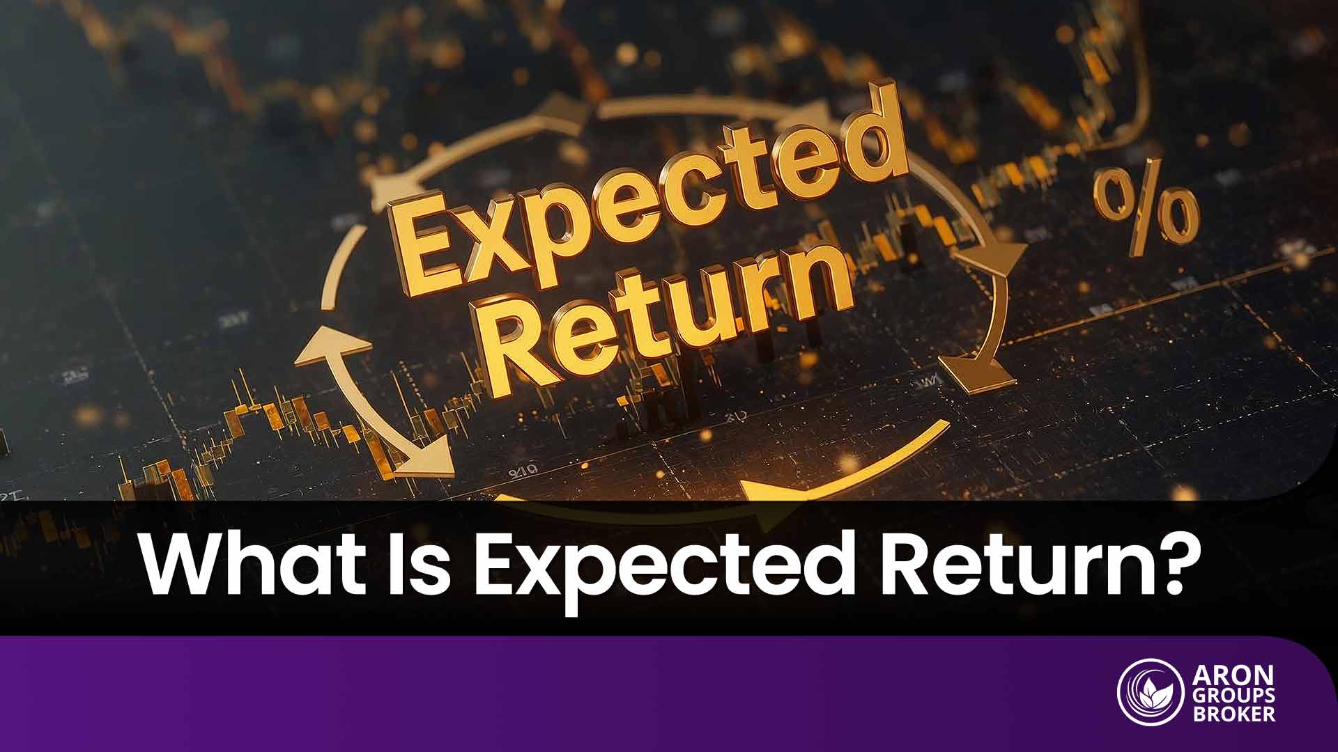
In financial markets, that tool is the concept of expected return. This metric is a statistical estimate that helps us make more rational choices among various investment options. Expected return doesn’t tell us exactly what will happen in the future, but it provides a logical outlook based on different probabilities and scenarios.
Ahead, we will explore in detail what this concept is and why it is crucial for every investor, from novice to professional.

- Always calculate expected return net of costs; commissions/fees, the bid–ask spread, and taxes reduce your realized return.
- Align liquidity with your investment horizon; an asset you can’t liquidate promptly at a fair price effectively delivers no usable return for short-term objectives.
- Use a range rather than a single point estimate (e.g., 8–12%); all forecasts carry uncertainty.
- Don’t treat probability weights as fixed; update scenario weights as new information arrives (i.e., Bayesian updating).
What Is Expected Return and Why Is It Important?
According to Wallstreetperp, expected return is the most logical forecast of the profit an investor can anticipate from an asset or an investment portfolio. This figure is a statistical forecast, not a guarantee. To calculate it, we consider all possible outcomes (different scenarios) of an investment and multiply each by its probability of occurrence. The sum of these values is the expected rate of return.
The importance of this concept can be summarized in three key applications:
- Comparison Tool: It provides a single, standardized metric that allows you to fairly compare different investment opportunities, each with its own unique risks and potential returns.
- Informed Decision-Making: It helps you evaluate whether accepting the risk of a particular investment is justified by the profit you expect to gain. This is the foundation of understanding the risk-return tradeoff.
- Financial Planning: This metric allows you to build an investment portfolio that aligns with your financial goals and helps you assess whether you are on the right track to achieve them (indeed).
Example
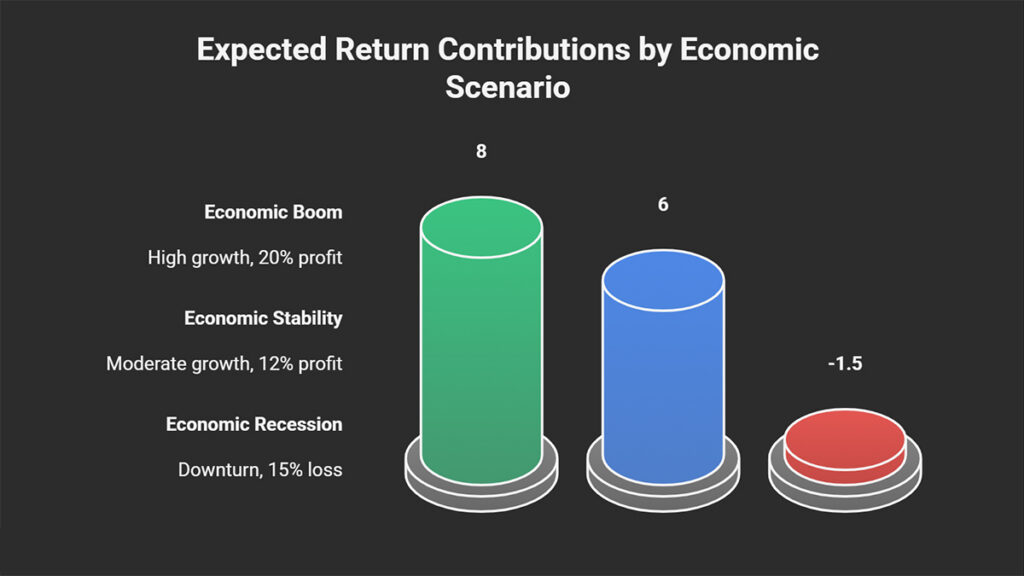
Imagine you want to invest in the stock of a technology company. Your analysis suggests that the stock’s future performance depends on three primary economic scenarios:
- Economic Boom Scenario: There is a 40% probability of this, in which case the stock will yield a 20% profit.
- Economic Stability Scenario: There is a 50% probability of this, resulting in a 12% profit.
- Economic Recession Scenario: There is a 10% probability of this, leading to a 15% loss.
To find the expected return, we calculate the contribution of each scenario to the final result:
- The boom scenario’s contribution to your overall return is 8 percentage points (since 40% of 20% is 8%).
- The stability scenario adds 6 percentage points to your return (since 50% of 12% is 6%).
- The recession scenario subtracts 1.5 percentage points from your return (since 10% of a 15% loss is a 1.5% loss).
Now, we combine these contributions: 8 percentage points from the first scenario, plus 6 points from the second, minus 1.5 points from the third. The final result is 12.5%.
Therefore, your expected return from this investment is 12.5%. Although your actual return may be a 20% profit, a 12% profit, or a 15% loss, the 12.5% figure represents the most logical, weighted-average estimate of the stock’s future performance.

In international portfolios, expected returns depend not only on the performance of the underlying assets but also on currency exchange rate volatility. This factor often overlooked by retail investors.
Expected Return vs. Realized Return: A Practical Example
The key difference between expected return and realized return lies in their time perspective:
- Expected Return: This is a forward-looking, forecast-based figure. It is calculated based on analysis, financial models, and probabilities, representing our most logical estimate of an investment’s future performance.
- Realized Return: This is a backward-looking, fact-based figure. It is the actual profit or loss that you see in your account after an investment period has passed.
In essence, expected return is your roadmap, while realized return is the path you actually traveled. The gap between these two figures arises from unforeseen events and the market’s inherent risks.
These risks can affect the entire market (systematic risk, such as an economic crisis) or be specific to a particular company (unsystematic risk, such as the success or failure of a new product).
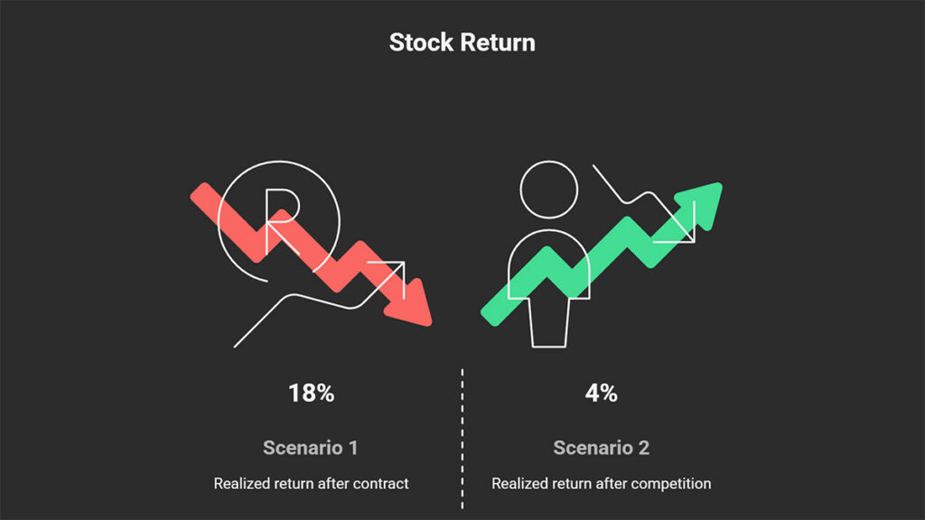
Example: Let’s return to the previous example where we calculated the expected return for a technology company’s stock to be 12.5%. Now, assume a year has passed, and you are reviewing the investment’s actual performance. Two different scenarios could have occurred:
- Scenario 1: The company signs a large, unexpected contract, causing its stock price to surge. At the end of the year, you have earned an 18% profit.
- Scenario 2: A strong competitor enters the market, reducing the company’s profitability. At the end of the year, you have earned only a 4% profit.
In both situations:
- Your Expected Return was: 12.5% (your initial forecast)
- Your Realized Return is: 18% (in the first scenario) or 4% (in the second scenario)
This example clearly shows that while expected return is a powerful analytical tool for decision-making, it can never predict the future with certainty. The realized return is what ultimately impacts your bottom line.
Formulas for the Expected Rate of Return
According to the Corporate Finance Institute (CFI), there are two primary and widely used formulas for calculating the expected rate of return, each applied in different situations.
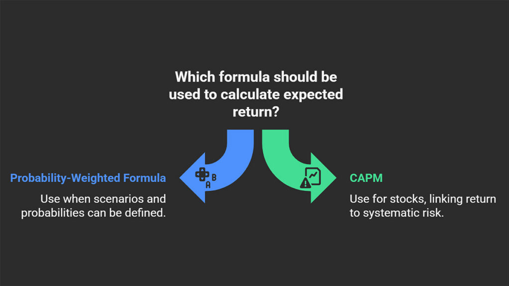
The Probability-Weighted Formula
This is the most fundamental and direct method for calculating expected return. We use this formula when we can define several plausible future scenarios for an investment and assign a probability of occurrence to each one.
Formula:
E(R)= ∑(Ri × Pi)
The components of this formula are:
- E(R): The final expected return.
- Rᵢ: The return (profit or loss) expected in scenario ‘i’.
- Pᵢ: The probability of scenario ‘i’ occurring.
- Σ (Sigma): This symbol represents the “summation,” meaning we add together the results of (Return × Probability) for all scenarios.
The Capital Asset Pricing Model (CAPM)
This formula is a cornerstone of professional financial analysis, particularly for stocks. The CAPM links the expected return of an asset to its systematic risk, the risk that is tied to the overall market and cannot be eliminated through diversification.
Formula:
E(Ri)= Rf + βi (E(Rm) − Rf)
The components of this formula are:
- E(Rᵢ): The expected return of the specific stock.
- Rբ: The risk-free rate (e.g., the yield on government bonds).
- βᵢ (Beta): The sensitivity or volatility of the stock relative to the overall market.
- E(Rₘ): The expected return of the overall market (e.g., a stock market index).
Methods for Calculating Expected Return in Investing
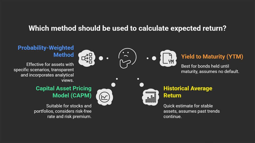
There is no single formula for calculating the expected rate of return for all assets. The best method depends on the asset type, the information available, and the depth of your analysis. Below, we review three primary approaches.
The Probability-Weighted Method
This is the most fundamental and transparent way to understand the concept of expected return. This approach is particularly effective for assets whose future is tied to a few specific scenarios, such as the stock of a particular company or a project.
The process is straightforward:
- Define Possible Scenarios: Identify different potential futures (e.g., economic boom, stability, or recession).
- Estimate Probabilities: Assign a percentage probability to each scenario (the sum of all probabilities must equal 100%).
- Forecast Returns: Estimate the return for each scenario.
- Calculate the Weighted Average: Multiply each scenario’s return by its probability and then sum the results.
This is the same method detailed in previous examples, and it allows you to directly incorporate your analytical views into the calculation.
The Capital Asset Pricing Model (CAPM)
The CAPM is one of the most famous formulas in finance, used specifically to calculate the expected return for stocks and investment portfolios. The core logic of the CAPM is that an asset’s expected return should be equal to the return on a risk-free investment, plus a risk premium that is proportionate to the asset’s systematic risk.
Example: Assume the risk-free rate is 5%, the market risk premium is 7%, and the beta of your target stock is 1.2. The expected return for this stock would be:
E(R)= 5% + 1.2 × (7%)= 5% + 8.4%= 13.4%
This figure indicates that, given the stock’s higher risk (a beta of 1.2), investors would expect a return of 13.4% to be compensated for taking on that additional risk.
Other Quick and Approximate Methods
In addition to the two main methods above, other approaches exist for specific situations:
- Historical Average Return: For stable and mature assets, the average return over the past several years can be used as a quick estimate for the future. However, this method assumes that the past will repeat itself, which is not always a valid assumption.
- Yield to Maturity (YTM) for Bonds: For debt instruments, YTM is the best approximation for the expected return, provided the bond is held until maturity and the issuer does not default.
- Multi-factor Models: More advanced models, such as the Fama-French model, exist that incorporate factors beyond market risk, such as company size and the book-to-market ratio, into their calculations.
The expected return for long-term projects can be calculated using a variable discount rate over time rather than a fixed rate, since market risk changes throughout economic cycles.
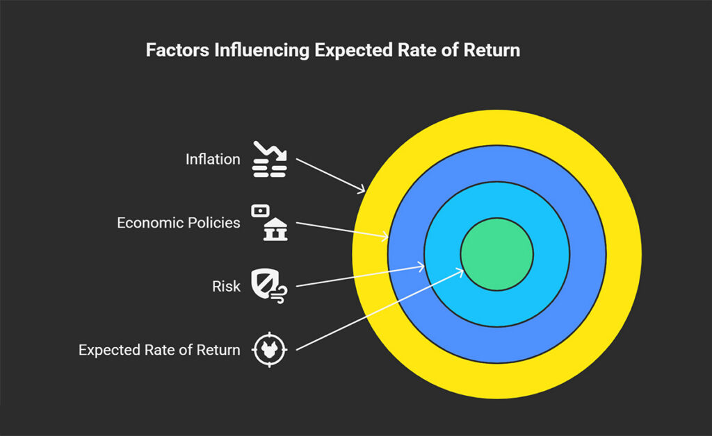
Factors Affecting the Expected Rate of Return
The expected rate of return is not a static figure; it is a dynamic variable that changes under the influence of various economic and financial forces. Understanding these factors helps investors align their expectations with market realities. The three key factors in this area are risk, economic policies, and inflation.
The Role of Systematic and Unsystematic Risk
In the world of finance, not all risks are created equal. Their primary difference lies in whether they can be eliminated through diversification:
Systematic Risk
Also known as “market risk,” this risk arises from macroeconomic factors such as financial crises, interest rate changes, or global recessions. This type of risk affects the entire market, and no investor, no matter how diversified their portfolio, can escape it.
Since investors are forced to bear this risk, they demand compensation for it. For this reason, the higher an asset’s systematic risk (as measured by the beta coefficient in the CAPM), the higher its expected rate of return will be.
Unsystematic Risk
This risk is specific to a particular company or industry, such as poor management, labor strikes, or a new product failure. The good news is that this type of risk can be easily mitigated by creating a well-diversified investment portfolio.
Modern financial theory holds that because this risk can be diversified away, the market does not offer an additional reward or return for bearing it. Therefore, the primary focus in determining expected return is on systematic risk.
The Effect of Interest Rates and Economic Policies
Monetary policies adopted by central banks have a profound and direct impact on the expected rate of return. The most important tool in this regard is the interest rate:
- Direct Effect: An increase in interest rates directly raises the risk-free rate (Rf) in the CAPM formula. This means the baseline return that investors expect from any investment increases.
- Indirect Effect: Higher interest rates mean higher borrowing costs for companies. This can reduce their profitability and put downward pressure on their stock prices. Therefore, when a central bank raises interest rates, investors’ expectations for market profits also change.
How Inflation Reduces the Real Expected Return
Inflation is the silent thief of purchasing power. The return that is typically calculated and quoted in the market is the nominal return. However, what matters to you as an investor is the real return, that is, the return after accounting for the effects of inflation.
The relationship between the two is very simple (the Fisher effect):
Real Return ≈ Nominal Return − Inflation Rate
Example: Imagine your expected return from an investment is 10%. If the annual inflation rate is 7%, your purchasing power has only increased by about 3%. This distinction is especially critical in long-term financial planning, such as for retirement, because your primary goal is to preserve and increase your purchasing power over time, not just the numerical value of your capital.
Expected Return in Different Markets
The concept of expected return is applicable across all financial markets, but its calculation method and the factors that influence it differ for each market.
How to Calculate the Expected Rate
the expected rate of Return for Stocks
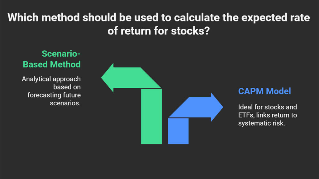
There are two primary approaches to calculating the expected rate of return for stocks:
- The CAPM Model: As previously explained, this model is ideal for stocks and Exchange-Traded Funds (ETFs) that are analyzed within the context of the broader market. This method directly links the expected return to the stock’s systematic risk (its beta coefficient).
- The Scenario-Based Method: This is a more analytical approach based on forecasting different future scenarios for a company (such as a new product launch, management changes, or quarterly earnings results) and assigning a probability to each.
Professional investors often use a combination of these methods along with fundamental analysis of the company.
Example (CAPM Model):
Let’s assume we want to calculate the expected return of a company’s stock using the CAPM and have the following information:
- Risk-Free Rate (Rf): 4%
- Expected Market Return (Rm): 10%
- Stock’s Beta Coefficient (β): 1.2 (meaning the stock is 20% more volatile than the overall market).
Calculation Steps:
- First, we calculate the “market risk premium”, which is the difference between the market return and the risk-free rate:
10% − 4%= 6%
- Next, we multiply this premium by the stock’s beta to account for its specific risk:
6% × 1.2= 7.2%
- Finally, we add the risk-free rate to this result to get the total expected return:
4% + 7.2%= 11.2%
Conclusion: This calculation shows that, given the stock’s higher risk (beta of 1.2), investors would rationally expect a return of 11.2% as compensation for taking on that additional risk.
The expected return can be derived not only from historical data but also from implied returns inferred from option prices.
What Factors Influence the Expected Return of Bonds and Debt Instruments?
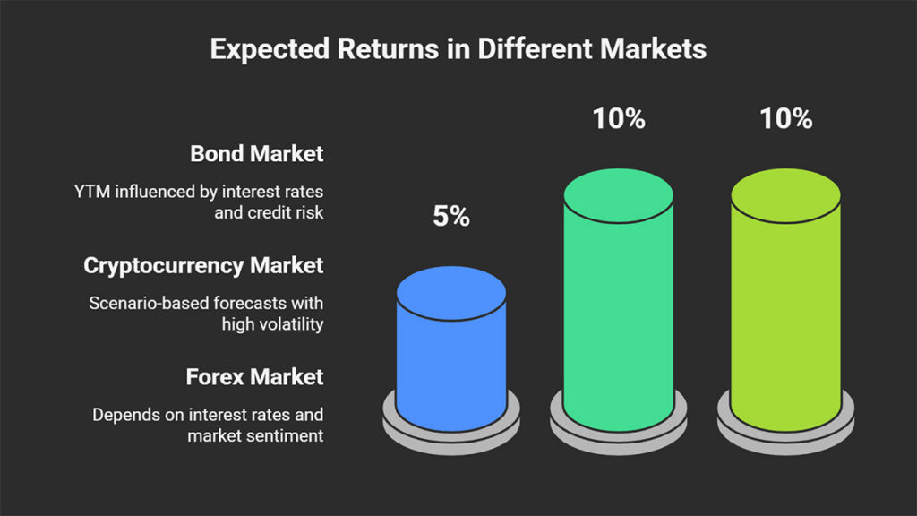
For bonds, the expected return is typically measured by the Yield to Maturity (YTM). This metric tells you the total return you will earn (including all periodic interest payments and the principal) if you hold the bond until its expiration date.
This return depends on several key factors:
- Market Interest Rates: Changes in interest rates affect the price of existing bonds and, consequently, their YTM.
- Issuer’s Credit Risk: The higher the issuer’s default risk, the higher the YTM investors will demand as compensation.
- Coupon Rate and Purchase Price: If you buy a bond below its face value (at a discount), your YTM will be higher than its stated coupon rate.
The YTM calculation is based on the assumption that you hold the bond to maturity and the issuer makes all payments on time.
Example: Imagine a company issues a bond with a face value of $1,000 and an annual coupon rate of 5%. This means it pays $50 in interest each year.
Now, suppose interest rates in the market rise, and new bonds are being issued with a 7% yield. Naturally, no one would want to buy the old 5% bond at its full price.
To remain attractive, the market price of the old bond will fall. Let’s say you buy it for $950.
The result for you:
- You still receive the $50 annual coupon payment.
- At the maturity date, the company will pay you the full $1,000 face value, which is $50 more than what you paid for it.
This extra profit ($50) causes your Yield to Maturity (YTM), as the new buyer, to be higher than the 5% coupon rate. This example clearly shows how the purchase price of a bond directly impacts your expected return.
The Role of Expected Return in Analyzing Cryptocurrencies and Forex
Calculating expected return in highly volatile markets like cryptocurrencies and forex is much more challenging because these assets do not generate intrinsic cash flows (like stock dividends or bond coupons).
- Cryptocurrency trading: In this market, analysts typically use the scenario-based method to forecast prices. They define different scenarios based on major news (such as new regulations or technical updates) and assign a probability to each outcome (e.g., a price increase or decrease). Given the market’s high volatility, the range of potential profits and losses is vast, and the probability of sudden, extreme events (both positive and negative) is high.
- Forex Trading: The expected profit from currency trades depends on two main factors: the interest rate differential between the two countries and what traders believe will happen to the exchange rate in the future. Additionally, to make better forecasts, traders constantly monitor the overall state of the economy, major geopolitical events, and general market sentiment to estimate potential profits or losses.
Example: A trader predicts there is a 60% probability that a cryptocurrency’s price will rise by 30% and a 40% probability that it will fall by 20%:
E(R)= (60%×30%) + (40%×−20%)= 18% − 8%= 10%
In this case, the trader’s expected return from this trade is 10%.
Practical Investment Strategies Using Expected Return
Expected return helps you formulate specific strategies for portfolio construction, risk management, and achieving your personal financial goals.
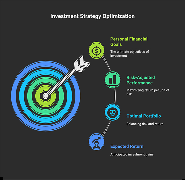
Selecting an Optimal Portfolio Based on Expected Return and Risk
The primary goal of investment portfolio management is to find the best possible combination of assets. An optimal or “efficient” portfolio has one of the following two characteristics:
- It offers the highest possible expected return for a given level of risk.
- It carries the lowest possible risk for a given level of expected return.
This idea is the foundation of Modern Portfolio Theory. By combining assets that behave differently from one another (e.g., stocks and bonds), you can optimize the overall risk of your portfolio without sacrificing returns. A precise evaluation of this combination requires calculating the portfolio’s overall risk.
Example: Imagine you must choose between two different investment portfolios:
- Portfolio A:
- Expected Return: 12%
- Risk Level (Volatility): High
- Portfolio B:
- Expected Return: 12%
- Risk Level (Volatility): Medium
Conclusion: In this case, Portfolio B is the optimal choice. Although both portfolios target the same expected return, Portfolio B gets you to that goal with less risk and volatility. This is a perfect example of optimizing a portfolio to minimize risk for a specific level of return.
Using Expected Return to Maximize Risk-Adjusted Performance
Expected return alone is not enough; it must be weighed against the risk you take to achieve it. In other words, which investment is truly “worth the risk?”
To answer this question, we use the Sharpe Ratio, which measures an investment’s excess return per unit of risk. The higher the ratio, the better the choice.
Example: Suppose you are deciding between two investment funds, both with an expected return of 10%. The risk-free rate is 3%.
- Fund A: Has a higher risk (standard deviation) of 15%.
- Fund B: Has a lower risk (standard deviation) of 10%.
Now, let’s calculate the Sharpe Ratio for each:
- Sharpe Ratio for Fund A = (10% – 3%) / 15% = 0.47
- Sharpe Ratio for Fund B = (10% – 3%) / 10% = 0.70
Conclusion: Even though both funds have the same expected return, Fund B is the smarter choice because it delivers that return with less risk. This strategy helps you maximize your return for the amount of risk you take.
Aligning Expected Return with Personal Financial Goals
This is the most critical step in using expected return: turning numbers and figures into an actionable plan for your life. This concept helps you answer the key question: “Is my investment path leading me to my goals?”
Example: An individual plans to retire in 20 years and, based on their calculations, needs an annual return of 9% for a comfortable retirement (this is their required rate of return).
- Analyze the Current Situation: They calculate the expected return of their current investment portfolio and find it to be 6%.
- Identify the Gap: There is a 3% gap between their required return (9%) and their expected return (6%).
- Make a Decision: This analysis forces them to choose one of the following options:
- Increase their monthly savings.
- Adjust their investment portfolio toward assets with a higher expected return (and, of course, higher risk).
- Re-evaluate their retirement goals (e.g., by retiring a few years later).
Key Takeaway: For long-term goals like retirement, always base your plans on the real expected return (after deducting inflation) to ensure your purchasing power is preserved over time.
Limitations and Criticisms of the Expected Rate of Return
Although the expected rate of return is a key tool in financial decision-making, it is not a flawless forecast, and blind reliance on it can be misleading. Understanding its limitations is as important as learning how to calculate it.
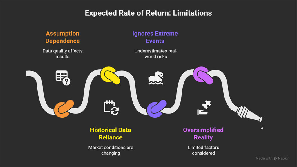
The most significant criticisms are as follows:
It Is Based on Assumptions (The “Garbage In, Garbage Out” Principle)
The quality of the expected return figure is entirely dependent on the quality of the data and assumptions used as inputs. An incorrect forecast about the probability of a scenario, an inaccurate estimate of a stock’s beta, or an unrealistic market risk premium can render the final result completely invalid.
Past Performance Is No Guarantee of Future Results
Many models rely on historical data (such as the average returns of previous years) to estimate future returns. However, market conditions are constantly changing. A company’s success over the past decade provides no guarantee that it will be repeated in the future, as it may face new competition, emerging technologies, or regulatory changes.
It Ignores Rare and Extreme Events (The “Black Swan” Problem)
Standard financial models typically assume a normal distribution for returns, meaning they consider the probability of extreme events (like sudden market crashes) to be very low. In the real world, financial crises, pandemics, or wars, often called “Black Swan” events, occur and can cause the actual return to be completely different from what the models predicted.
It Oversimplifies Reality
Models like the CAPM reduce the complex reality of the market to one or a few limited factors. In contrast, many more factors, such as company size, industry conditions, and the quality of management, also influence a stock’s return. This oversimplification can lead to inaccurate estimates of the expected return.
Methods and Alternatives for Improving Expected Return Analysis
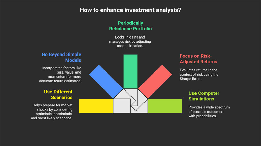
Here are several key approaches you can use to enhance your analysis:
Use Different Scenarios and Stress Testing
Instead of relying on a single average, define several different future scenarios: optimistic, pessimistic, and most likely. This process, also known as “stress testing,” helps you see how vulnerable your investment portfolio is under extreme conditions. This approach better prepares you for potential market shocks.
Go Beyond Simple Models (Using Multi-factor Models)
The CAPM only considers market risk. However, more advanced multi-factor models incorporate other factors that are also known to influence stock returns, including:
- Size: Smaller companies have different growth potential.
- Value: Stocks that are trading below their intrinsic value.
- Momentum: Stocks that have demonstrated a strong upward trend.
Using these models can lead to a more accurate estimate of the expected rate of return.
Periodically Rebalance Your Portfolio
Portfolio rebalancing means periodically buying and selling assets to return to your original asset allocation and risk level. For example, suppose your stocks have grown significantly and their weight in your portfolio exceeds your initial target. In that case, you can control your portfolio’s risk by selling a portion of it and buying other assets. This is a smart strategy for locking in gains and managing risk.
Focus on Risk-Adjusted Returns (The Sharpe Ratio)
A high expected return is not necessarily a good choice if it comes with exceptionally high risk. You should always evaluate a return in the context of its risk. According to Investopedia, the best tool for this is the Sharpe Ratio, which shows how much excess return you receive for each unit of risk you take. Comparing the Sharpe Ratio of different options helps you make a more intelligent choice.
Use Computer Simulations (Monte Carlo)
A Monte Carlo simulation is a computer-based method that models thousands of potential futures for your investment portfolio based on its risk and return characteristics. The output is not a single number, but a complete picture of a wide spectrum of possible outcomes and the probability of each. This provides a much deeper insight than a simple expected return figure.
Conclusion
Expected return is a powerful and essential statistical tool in every investor’s toolkit. This concept helps us move beyond guesswork and provides a logical framework for evaluating and comparing different investment opportunities. Whether through the simple scenario-based method or by using more advanced financial models like the CAPM, this metric can clarify our decision-making path.
However, it is crucial to remember that expected return is a forecast, not a guarantee. For intelligent decision-making, this figure should never be used in isolation. This metric must always be applied alongside a thorough analysis of factors such as risk, inflation, and overall macroeconomic conditions.