


Modern financial markets depend more than ever on precision, speed, and data. The enormous volume of information and the growing complexity of price behaviour mean that decisions based only on intuition or experience are no longer sufficient.
Quantitative investing emerged as a modern response to this environment. It is a method that combines data science, statistics, and programming to build trading strategies. This approach is not a replacement for human judgment. It is a tool that brings structure, discipline, and accuracy to a market that changes every second.
This guide explores the foundations of quantitative investing and quantitative trading.

- Quantitative trading uses mathematical and statistical models to identify opportunities and reduce emotional decision-making.
- A quantitative trading system relies on four core components: strategy design, backtesting, execution, and risk management.
- Success in quantitative trading requires a combination of skills across mathematics, programming, finance, and critical thinking.
- No strategy performs well in every market environment; quantitative trading also faces performance cycles.
What Is Quantitative Investing and How Does It Work?
According to reputable sources such as Investopedia, quantitative investing is a scientific, data-driven approach to financial markets. It relies on numbers, models, and logic rather than sentiment or speculation. In this framework, decisions are made using statistical analysis and computer algorithms, helping to minimise the influence of human emotion.
In simple terms, computers perform the analytical work that traders once did manually but much faster, more accurately, and without emotional bias. By analysing historical market data, quantitative models look for patterns in price movements, trading volume, and market indicators to forecast future behaviour.
For example, if historical data shows that technology stocks tend to rise when interest rates fall, a quantitative model can automatically open long positions based on this relationship.
Why Quantitative Investing Matters Today
Modern financial markets move at extraordinary speed and generate massive volumes of data. In this environment, traditional analysis is no longer sufficient. Quantitative investing has therefore become an essential, scientific, data-driven approach that removes emotional bias and bases decisions on logic and computation.
Its importance comes from several structural advantages:
- High data volume: Billions of financial, economic, and news-based data points are generated every day. Quantitative models, supported by artificial intelligence and statistical analysis, can process these datasets and uncover hidden patterns.
- Market speed: Prices can shift within seconds. Quantitative trading algorithms analyse conditions and execute orders in fractions of a second, far faster than any human.
- Greater efficiency: Quantitative models can detect relationships that human analysts often overlook, for example, the correlation between changes in crude oil prices and transportation stocks.
- Removal of cognitive bias: Quantitative trading isolates decision-making from emotions such as fear or greed, leading to more disciplined and consistent actions.
- High scalability: These systems can operate across multiple markets and instruments simultaneously, without human or time limitations.
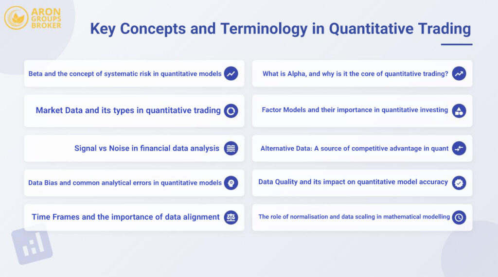
Key Concepts and Terminology in Quantitative Trading
Understanding quantitative trading requires familiarity with a set of core concepts. These terms form the shared language between analysts, traders, and algorithm developers. Knowing them helps you understand the logic behind automated decisions and numerical models.
Alpha: The Core Objective of Quantitative Strategies
Alpha represents the excess return a strategy generates relative to the market or a benchmark index. If the market returns 10% and your strategy delivers 12%, the alpha is 2%.
In quantitative trading, generating alpha is the central goal of discovering hidden patterns in data that can outperform the broader market. Alpha reflects the “intelligence” or effectiveness of the strategy.
Beta and Systematic Risk in Quantitative Models
Beta measures the sensitivity of an asset or portfolio to overall market movements:
- Beta = 1: moves in line with the market.
- Beta > 1: more volatile than the market.
- Beta < 1: less volatile than the market.
- Negative beta: moves in the opposite direction.
In quantitative frameworks, beta is used to assess systematic risk and maintain a balanced risk–reward structure across portfolios.
Factor Models and Their Role in Quantitative Investing
Factor models explain asset returns based on economic, financial, or behavioural drivers. A well-known example is the Fama-French three-factor model, built on market exposure, company size, and value-to-market ratios.
These models form the foundation of smart portfolio construction by identifying common risk sources and the true origins of return.
Market Data and Its Types in Quantitative Trading
Market data is the raw material for quantitative models. It includes open, close, high, low prices, volume, and order flow.
Main categories include:
- Tick data: the most granular view of every transaction;
- Minute data: aggregated price and volume per minute;
- Daily, weekly, and monthly data: suitable for medium- and long-term analysis.
The choice of data depends on the strategy’s time horizon and execution intensity.
Alternative Data: A Competitive Edge in Quant
Alternative data refers to non-traditional datasets collected from outside financial markets, such as:
- social-media sentiment analysis;
- satellite imagery;
- credit-card transaction flows;
- website traffic patterns.
These datasets offer early signals on market behaviour before trends appear in price.

In quantitative investing, emotion is not eliminated. It is treated as a variable to measure, model, and weight.
Signal vs Noise in Financial Data
In data analysis, a signal represents meaningful information that helps predict future market movements, whereas noise refers to random, irrelevant fluctuations.
The skill of a quantitative trader lies in separating signal from noise using statistical filters, moving averages, or machine-learning methods.
Data Quality and Its Impact on Model Accuracy
Even the strongest model fails when the data is weak. High-quality data must be:
- precise and error-free;
- complete and consistent across sources;
- updated promptly.
Data cleaning and preparation are as crucial as model design in quantitative trading.
Data Bias and Common Analytical Errors in Quant Models
Bias occurs when data gives a misleading view of the market. Common examples include:
- Survivorship bias: excluding delisted or bankrupt companies;
- Look-ahead bias: using information in analysis that was not available at the time;
- Selection bias: biased or non-random sampling.
Correcting these issues is essential for models to reflect real market conditions.
Time Frames and the Importance of Data Alignment
Time frames indicate the period over which data is collected, from milliseconds to months. Selection depends on strategy type:
- Fast strategies rely on tick or minute data.
- Long-term investing prefers daily or monthly data.
Data alignment ensures time stamps across datasets match, allowing the model to analyse accurately.
Normalization and Scaling in Quantitative Modelling
Financial data often varies in magnitude. Normalisation puts all variables on a comparable scale. Common techniques include:
- Min-max scaling: converts values to a 0–1 range;
- Standardisation: adjusts data to mean zero and standard deviation one;
- Log normalisation: reduces the effect of extreme volatility.
These methods improve model accuracy and prevent larger-scale variables from dominating results.
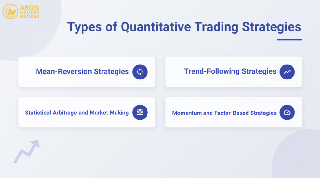
Types of Quantitative Trading Strategies
Quantitative trading is built on data, statistics, and numerical logic. Depending on the analytical approach and the objective, strategies take different forms. The following section summarises the most common quantitative strategies in a practical, concise way.
Trend-Following Strategies
Trend-following assumes that prices tend to move in a consistent direction. If an asset is rising, it may continue to rise; if it is falling, the decline may extend. The goal is to identify the trend and follow it, not to predict reversals.
Key steps usually include:
- detecting the trend using tools such as moving averages or the Average Directional Index (ADX);
- entering positions in the direction of the trend;
- exiting when signs of weakness or trend reversal appear;
- managing risk through stop-loss levels.
These strategies perform well in strong trending markets but may generate false signals during sideways or range-bound conditions.
Mean-Reversion Strategies
The core idea of mean reversion is simple: when a price moves too far from its historical average, it tends to revert to it. Prices often oscillate around an equilibrium level, and extreme deviations typically correct over time.
Common features include:
- identifying deviations from historical averages;
- entering positions against the current move (buying at lows, selling at highs);
- waiting for the price to move back toward the mean;
- using tools such as Bollinger Bands or the RSI to detect reversal points.
This approach works well in quiet or non-trending markets, but during strong trends it can lead to losses.
Momentum and Factor-Based Strategies
Momentum refers to the continuation strength of price movement. This strategy assumes that past winners tend to remain winners, while past losers often continue to underperform.
In practice:
- assets with strong recent performance are bought, and weaker assets are sold;
- positions are held as long as price momentum persists;
- Indicators such as rate of change (ROC) or periodic average returns measure momentum strength.
Factor-based strategies examine how specific characteristics such as company size, value, momentum, quality, or volatility affect returns.
These models aim to build diversified portfolios with higher risk-adjusted returns by combining different factors.
Statistical Arbitrage and Market Making
Statistical arbitrage (stat-arb) seeks temporary pricing anomalies between related assets. For example, if two stocks historically move together but suddenly diverge, a quantitative model may buy the undervalued stock and sell the overvalued one, expecting prices to converge.
Its main principles include:
- identifying statistical relationships between assets;
- opening long and short positions simultaneously;
- exiting once prices return to their historical mean;
- applying strict risk controls if convergence does not occur.
Market making, by contrast, is a strategy that provides both bid and ask prices and profits from the spread. It requires extremely fast execution and robust technical infrastructure, and is typically implemented through high-frequency trading (HFT) systems.
In quantitative trading, the real risk lies in model variance, not market variance.
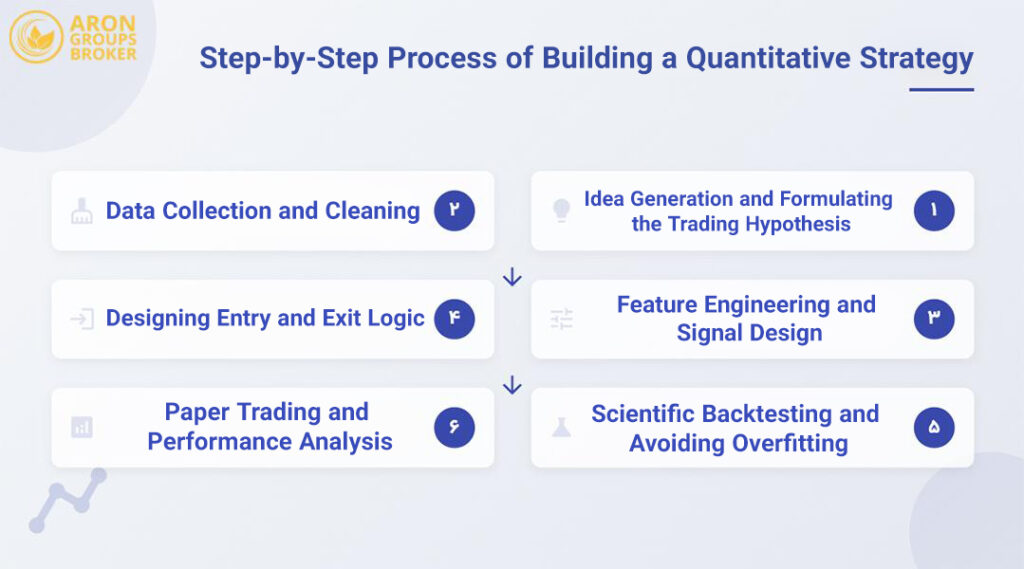
Step-by-Step Process for Building a Quantitative Strategy
The following section outlines the core stages of building a quantitative trading strategy in a simple but precise way.
Idea Generation and Formulating a Trading Hypothesis
Every successful strategy begins with an idea, a hypothesis grounded in economic logic or observed market behaviour. The goal is to convert a general intuition into a testable statement.
Key steps in forming a quantitative hypothesis:
- Market observation: identifying patterns, recurring behaviours, or pricing anomalies.
- Reviewing past research: studying economic theories and validated trading strategies.
- Formulating the hypothesis: expressing a clear, measurable idea, such as
“Stocks with lower P/E ratios outperform the market over the long term.” - Defining variables and test design: selecting relevant factors and determining how they will be evaluated in the dataset.
A good hypothesis must be simple, logical, and measurable.
Data Collection and Cleaning
Data is the fuel of quantitative trading. Without accurate and clean datasets, no model can be trusted. This stage involves collecting historical, fundamental, macroeconomic, or even alternative data (such as website traffic or social-media sentiment) and preparing it for analysis.
Core steps:
- identifying data sources (e.g., Bloomberg, Yahoo Finance, specialist databases);
- gathering data across sufficient time periods;
- cleaning errors, outliers, and missing values;
- aligning timestamps across different sources;
- normalising data for comparability.
The cleaner the dataset, the more reliable the backtest. Poor data can invalidate even the most sophisticated model.
Feature Engineering and Signal Design
Here, raw data is transformed into features and trading signals, the indicators that guide model decisions.
Main steps:
- selecting features relevant to the hypothesis (e.g., volume, volatility, past returns);
- engineering new variables from raw data (e.g., log returns, moving averages);
- generating signals, such as “Buy when RSI is below 30;”
- setting thresholds and evaluating each signal’s predictive power.
Quantitative models must be built on economically meaningful relationships, not on random patterns that appear only in historical data.
Designing Entry and Exit Logic
This step defines the operational framework of the strategy, including when to buy, when to sell, and under what conditions positions are held.
Core principles:
- defining entry rules (e.g., short-term moving average crosses above the long-term average);
- specifying exit rules (reversal signals or price targets);
- setting stop-loss and take-profit levels;
- outlining time-based rules for entering or holding trades.
The objective is to create a clear, code-ready logic that the algorithm can execute without ambiguity.
Scientific Backtesting and Avoiding Overfitting
Backtesting examines how a strategy would have performed on historical data. However, a careless backtest may produce misleading results.
Proper backtesting requires:
- splitting data into training, validation, and test sets;
- simulating trades according to the strategy’s rules;
- calculating metrics such as return, Sharpe ratio, and maximum drawdown;
- checking for overfitting when the model fits past data perfectly but performs poorly in the future.
To ensure the strategy is genuinely robust, it must be tested across different datasets, time periods, and market conditions.
Paper Trading and Real-Market Validation
Once the model performs well on historical data, it must be tested in real-time conditions. This stage bridges theory and practice.
Main steps:
- Running paper trading simulations with no financial risk;
- Deploying the strategy with small position sizes to observe live results;
- Continuously monitoring performance and comparing it with backtest outcomes;
- Analysing discrepancies and adjusting parameters.
This stage reveals real-world factors such as slippage, execution delays, and regime shifts. Refining the model based on live data is essential before full-scale deployment.
In quantitative investing, AI only makes sense when its prediction error is lower than the variance of the actual data.
How to Evaluate a Quantitative Strategy: Key Performance Metrics
After building and deploying a quantitative strategy, the most important question is simple: Does it actually work?
To answer this, performance must be measured using scientific, reliable metrics, ones that evaluate not only returns but also the risk and stability behind those returns.
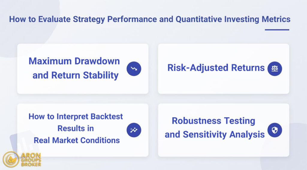
Risk-Adjusted Returns
In investing, the amount of profit is not the only thing that matters; the quality of that profit is equally important. Risk-adjusted return measures how much return a strategy generates relative to the risk taken.
Two strategies may show identical returns, but the one that achieved those returns with lower volatility is objectively stronger.
Key metrics include:
- Sharpe ratio: compares excess return to total volatility. A higher value indicates more efficient performance.
- Sortino ratio: similar to Sharpe but focuses only on downside volatility (losses).
- Calmar ratio: annual return divided by the maximum drawdown.
- Information ratio: evaluates the strategy’s outperformance relative to a benchmark.
These measures help determine whether a strategy is genuinely intelligent in managing risk, or whether the positive results are simply luck.
Maximum Drawdown and Return Stability
No strategy is free from declines. Maximum drawdown shows the worst peak-to-trough drop in portfolio value. For professional traders, this is a core measure of risk tolerance.
Return stability reflects how consistently a strategy performs over time. A model that earns strong returns but swings between large gains and losses is generally less attractive to investors.
Common stability metrics include:
- Standard deviation of returns: lower values indicate smoother performance.
- Coefficient of variation (CV): volatility relative to average return, used to assess consistency.
- Return stability index: a combined measure that evaluates overall uniformity.
In practice, strategies with moderate but stable returns often outperform models that generate high but erratic results.
Robustness Testing and Sensitivity Analysis
A strong strategy must remain reliable across different market conditions, not just during a favourable period. Robustness testing evaluates how well the model performs across multiple environments.
Sensitivity analysis reveals how dependent the strategy is on specific parameters. If small changes to a variable (such as stop-loss distance or moving-average period) dramatically alter performance, the model is unstable.
Common methods include:
- Testing across different time periods to check long-term consistency;
- Testing in different market regimes (bull, bear, sideways);
- Varying parameters to identify fragile points;
- Using simulated or alternative datasets to measure adaptability.
The goal is to ensure the strategy is based on real economic logic, not on patterns unique to historical events.
Interpreting Backtest Results in Real Market Conditions
Backtesting is similar to a flight simulator: useful, but never identical to real flight. Backtest results often appear better than live results because they exclude real-world frictions.
When interpreting backtests, consider:
- Backtest results are always more ideal than reality; live execution introduces error.
- Transaction costs and fees must be included, as they can significantly reduce returns.
- Low liquidity may prevent orders from filling at the expected price.
- Market structure evolves, requiring regular model updates.
- The backtest period must be long and diverse enough to be statistically valid.
Ultimately, backtesting alone is not enough. Paper trading and limited real-market deployment are essential for confirming whether the strategy can remain stable under live conditions.
Risk Management and Portfolio Optimisation in Quantitative Investing
The following section explains the four core components of risk management in quantitative investing.
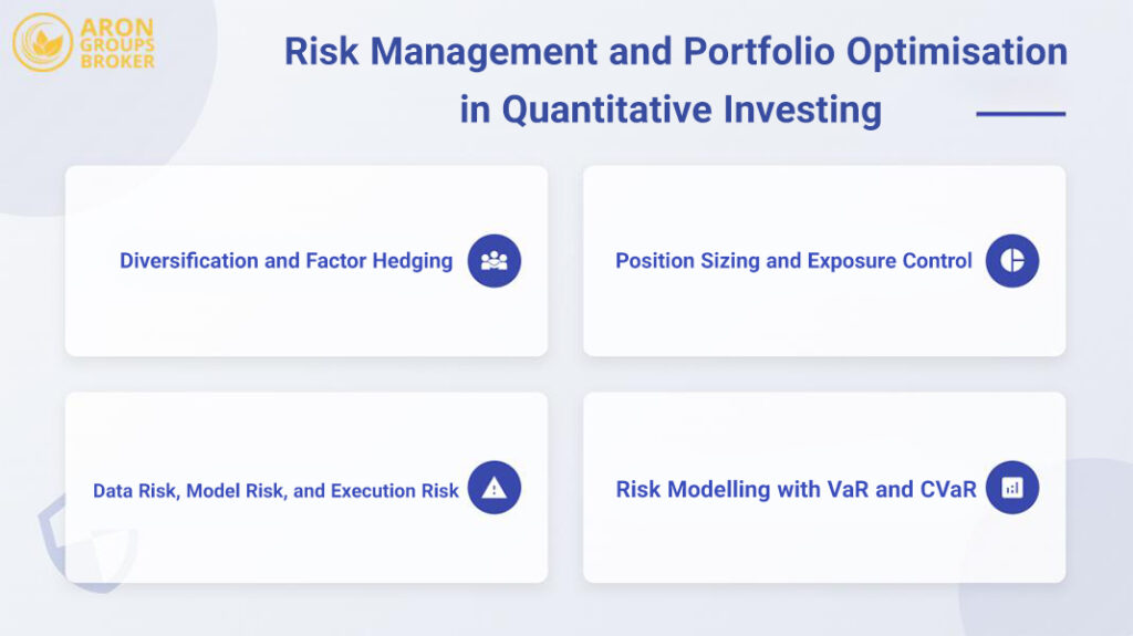
Position Sizing and Exposure Control
Position sizing determines how much capital is allocated to each trade. This decision must reflect the strategy design, account size, and risk tolerance.
If positions are too large, a single loss can erase accumulated gains. If they are too small, the strategy may fail to grow.
Common methods of position sizing include:
- Fixed percentage: allocating a specific percentage of capital (e.g., 2%) per trade;
- Fixed amount: investing a set monetary value in each position;
- Risk-based sizing: adjusting position size so that a stop-loss does not exceed a defined percentage of capital;
- Volatility-based sizing: smaller positions in volatile assets and larger positions in stable ones;
- Kelly formula: a mathematical method for determining the optimal position size based on win probability and payoff ratio.
Exposure control manages how much of the overall portfolio is exposed to market risk. If several assets behave similarly, rising and falling together, the portfolio should not be concentrated in all of them at once. This prevents the portfolio from becoming dependent on a single sector or market regime.
Diversification and Factor Hedging
Portfolio diversification spreads capital across different assets, markets, and strategies to reduce idiosyncratic risk, the risk related to a single company or sector.
Common forms of diversification include:
- Across asset classes: equities, bonds, commodities, and currencies;
- Geographic diversification: exposure to international markets;
- Time diversification: executing trades at different time intervals.
Factor hedging neutralises broad risk factors such as interest rates, market volatility, or currency movements. For example, if a portfolio is sensitive to interest-rate changes, futures or bonds in the opposite direction can offset this exposure.
Combining diversification with factor hedging creates portfolios with lower volatility and more stable performance.
Risk Modelling Using VaR and CVaR
To measure portfolio risk, we need to estimate potential losses under adverse conditions. Two widely used tools are:
- Value at Risk (VaR): estimates the maximum expected loss over a given time horizon at a specified confidence level.
Example: A one-day VaR at 95% confidence means there is a 5% chance the loss will exceed that amount. - Conditional Value at Risk (CVaR): the average loss in scenarios that exceed the VaR threshold; it measures the severity of extreme losses.
These metrics help evaluate vulnerability to major market shocks. They are easy to interpret and widely used, but should be combined with other tools, such as historical volatility and stress testing, for a complete risk profile.
Data Risk, Model Risk, and Execution Risk
In quantitative trading, market risk is not the only danger. Three additional risks can significantly impact performance:
- Data Risk: Incorrect, incomplete, or inconsistent data leads the model to make decisions based on false information.
Effective control requires continuous cleaning, validation, and sourcing from reliable providers. - Model Risk: Faulty assumptions, overfitting, or excessive complexity can produce backtests that fail in real markets.
The best defence is using simpler models, testing across diverse conditions, and continuously monitoring live performance. - Execution Risk: Real-market execution involves delays, slippage, and technical errors.
Fast, stable infrastructure and realistic cost assumptions (commissions, spreads, fees) are essential to manage this risk.
Technical Infrastructure and Tools Required for Quantitative Trading
The infrastructure behind quantitative trading depends on the strategy type, execution speed, and operational scale. However, it generally consists of four core components: hardware, software, data, and monitoring systems.
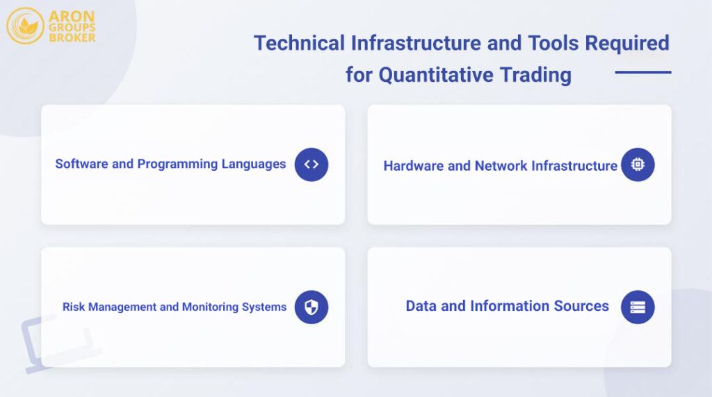
Hardware and Network Infrastructure
Hardware and network systems form the backbone of every quantitative trading setup.
If the system is slow or unstable, even the most accurate models can fail in live markets.
Key hardware components include:
- Servers: used for heavy computation and fast data processing;
- RAM: temporary storage for real-time data streams;
- Storage: for historical datasets and backtesting results;
- High-speed, stable network: essential for real-time data feeds and fast order execution;
- Backup systems: to protect data against outages or hardware failures.
In high-frequency strategies, even a few milliseconds of delay can be the difference between profit and loss. This is why many quantitative funds place their servers close to brokerage data centres (co-location) to maximise execution speed.
Software and Programming Languages
Software and programming languages are the primary tools for designing, testing, and deploying quantitative strategies. The right choice directly affects development speed, accuracy, and system efficiency.
Common programming languages in quantitative trading:
- Python: the most widely used language for data analysis and model development; libraries include Pandas, NumPy, and Scikit-learn;
- R: specialised for statistical modelling and advanced financial analysis;
- MATLAB: powerful for numerical computation and quantitative testing;
- C++: suitable for high-frequency trading due to very high execution speed;
- Java: a balanced option for building stable, scalable trading systems.
In addition to programming languages, platforms such as the Bloomberg Terminal, Refinitiv (formerly Reuters), and proprietary broker systems provide real-time market data and trade execution.
Data and Information Sources
In quantitative trading, data is the roadmap. Every decision is driven by data, so accuracy and reliability directly affect performance.
Types of data used in quantitative strategies:
- Market data: historical prices, trading volume, tick-level data;
- Fundamental data: financial statements, profitability metrics, and company ratios;
- Economic data: interest rates, inflation, GDP, and other macroeconomic indicators;
- Alternative data: non-traditional sources such as satellite imagery, web-search trends, or social-media sentiment;
- News and event data: the impact of economic, political, or corporate announcements.
These datasets come from providers such as Bloomberg, Reuters, Quandl, Yahoo Finance, or specialised data vendors. The key requirement is that data must be accurate, timely, and fully reliable.
Risk Management and Monitoring Systems
Once a strategy is live, continuous monitoring is essential to detect errors, instability, or unexpected behaviour. Risk-management and monitoring systems provide this layer of oversight.
Core components include:
- Monitoring dashboards: real-time views of trades, P&L, and risk levels;
- Alerts: automatic notifications triggered when risk thresholds are breached;
- Performance reports: daily or periodic evaluations of strategy behaviour;
- Stress testing: simulations showing how the portfolio reacts to extreme market conditions;
- Risk limits and circuit breakers: automated controls that halt trading if risk exceeds predefined limits.
These systems help traders maintain visibility, manage risk proactively, and take corrective action when needed.
Common Challenges and Mistakes in Quantitative Investing
The following section highlights the most important challenges quantitative traders must understand and avoid.
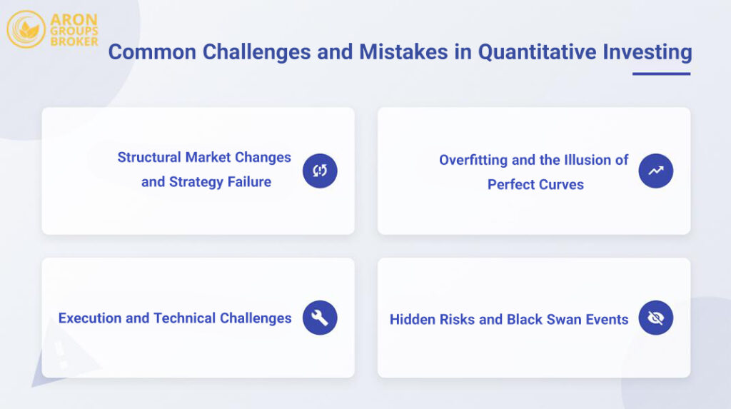
Overfitting and the Illusion of “Perfect” Backtests
One of the biggest traps in quantitative trading is overfitting. In this situation, a model becomes so closely tailored to historical data that it effectively “memorises” the past rather than learning patterns that persist in the future.
The backtest may appear flawless, with high returns, low risk, and a smooth upward curve, but this is often nothing more than a visually attractive chart, not a reliable strategy.
Structural Market Changes and Strategy Failure
Markets evolve continuously. Rules and patterns that worked in the past may become ineffective when conditions shift.
Regulatory changes, technological advancements, changes in trader behaviour, or global economic events can all cause a previously strong model to stop performing.
A quantitative strategy must be adaptable; otherwise, structural shifts can break it entirely.
Hidden Risks and Black Swan Events
Quantitative models always face risks that do not show up in historical data or backtests. These “hidden risks” only reveal themselves in real markets, often at the worst possible time.
In addition, black swan events, rare, unpredictable, high-impact shocks such as the 2008 market crash or the COVID-19 pandemic, can disrupt even the most sophisticated models.
Execution and Technical Challenges
Even the best-designed model can fail due to real-world operational issues. Live trading introduces challenges such as:
- software bugs;
- hardware failures;
- network delays;
- slow execution;
- slippage and liquidity constraints.
A strategy that works on paper may collapse if the technical infrastructure is not robust.
Conclusion
Quantitative investing succeeds when data science is combined with a fundamental understanding of market behaviour. Mathematical models reduce emotional bias and improve decision-making, but without human oversight, flexibility, and economic insight, they can easily drift off course.
In the end, the true strength of quantitative trading lies in balancing statistical logic with human judgment.