


Volatility Prediction tells you how “wild” the market may get next. It does not try to guess up or down. It estimates the potential magnitude of the moves. This matters in Forex, gold, and crypto, where prices can jump fast.
Volatility prediction helps you make smarter choices, set realistic stop losses, size positions safely, and pick the right strategy for the market mood.
In this article, you will learn practical ways to forecast volatility using indicators, GARCH models, and machine learning (ML). We keep it clear, numeric, and trader-focused.

- Volatility Prediction is about magnitude, not direction. High volatility means bigger swings, not bearish or bullish.
- Realised Volatility (ATR/HV) helps with stop-loss and position sizing. Implied (options/VIX) helps with event risk and sentiment.
- The gap between IV and realised volatility is a signal:
IV >> realised = event risk priced in.
Realised>> IV = risk may be underpriced.
- Volatility is useless unless it changes your sizing.
If ATR doubles, your stop usually widens, and your position size must drop to keep risk fixed.
What Is Volatility Prediction?
Volatility Prediction means estimating how much the price may move in the future (the next hour, the next day, or the next week). It is a risk forecast, not a direction call. Traders use it to manage leverage, decide whether to trend-trade or range-trade, and avoid trading into unstable conditions.
For example, if Gold (XAUUSD) usually moves $10 per day and suddenly starts moving $30, volatility has increased. The market is now riskier. Old stop losses fail. Position sizes must change.
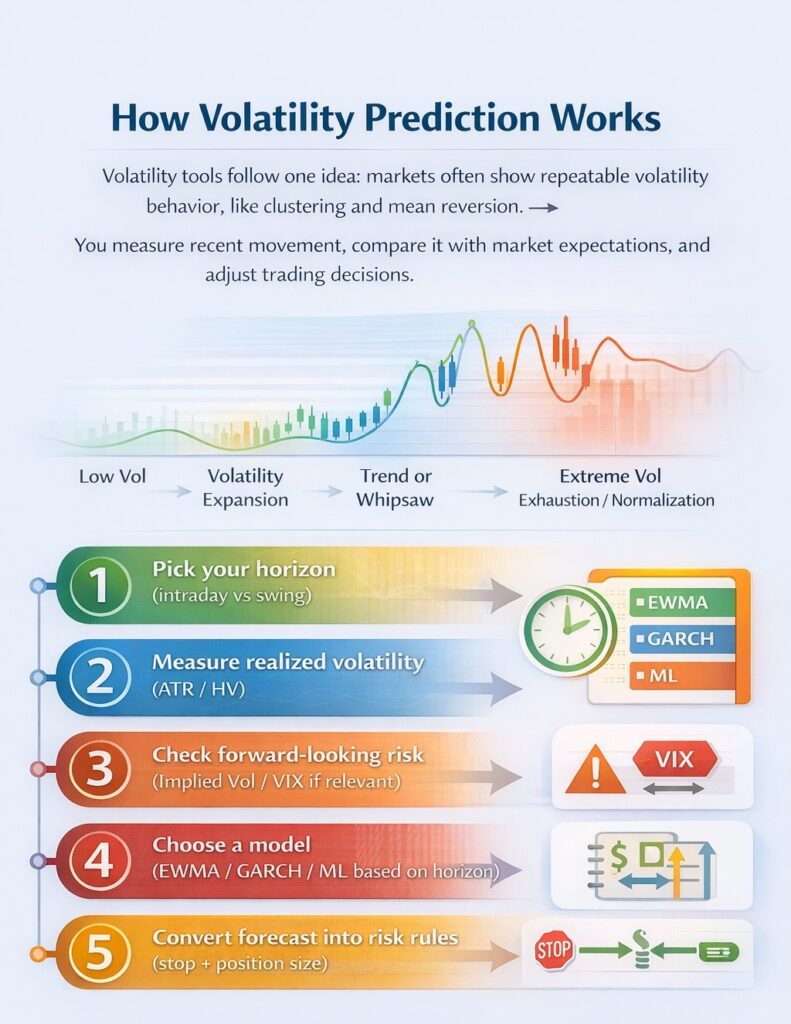
How Volatility Prediction Works?
Volatility tools follow one idea: markets often exhibit repeatable volatility behaviour, such as clustering and mean reversion.
You measure recent movement, compare it with market expectations, and adjust trading decisions.
Trader workflow (use this as a checklist)
- Pick your horizon (intraday vs swing)
- Measure realised volatility (ATR/HV)
- Check forward-looking risk (Implied Vol / VIX if relevant)
- Choose a model (EWMA/GARCH/ML based on horizon)
- Convert forecast into risk rules (stop + position size)
Types of Volatility in Financial Markets
Volatility is the extent to which a price moves over a given period. Traders care because it controls risk, stop-loss size, and position size.
In practice, most trading decisions use two volatility measures:
- Realised Volatility (past movement)
- Implied Volatility (expected future movement implied by options).

Key Point:
A market can be calm today (low realised volatility) but still be priced for a big move tomorrow (high implied volatility), especially before CPI, NFP, or a central bank decision.
Realised Volatility (Past-Based)
Realised volatility measures what actually happened in the past. It uses historical prices. It is used for risk control, not hype. Traders calculate it using the returns’ standard deviation or use the ATR as a simple proxy.
Numeric example:
If GBP/USD ATR(14) = 110 pips:
- The market has been moving about 110 pips per day recently.
- A stop loss of 25 pips is probably noise.
- A stop loss of 120–150 pips may be more realistic depending on the strategy.
Q: Why does realised volatility help?
A: Realised volatility helps because volatility tends to cluster. When price movements become large, they often stay large for a while due to ongoing market pressure and trader behaviour. This makes recent volatility a practical guide for short-term risk planning.
Implied Volatility (Expectation-Based)
Implied volatility (IV) is forward-looking. It comes from options prices. If traders expect larger moves, options become expensive, and IV rises. IV is useful for event risk and market sentiment.
Numeric example:
If S&P 500 IV rises from 14% → 22%:
- The market is pricing bigger swings ahead.
- This can happen even if the index is flat today.
- For gold, a higher IV before CPI often signals big move expected.
Key Point:
Implied volatility does not predict outcomes; It reflects expectations, which can be wrong.
Realised vs Implied Volatility Prediction (How to Use the Gap)
Realised volatility prediction uses past movement to estimate near-term risk. Implied volatility prediction uses options expectations to estimate future risk. They can disagree, and that difference is valuable.
How traders read the gap:
- IV >> Realised: market fears a future shock (event risk priced in).
- Realised >> IV: the market may be underpricing ongoing instability.
Numeric example:
Realised daily move = 0.6%, but IV implies 1.2%. Expect wider ranges ahead or higher uncertainty.
Realised Volatility Prediction Using Historical Prices
Predicting volatility using historical prices is based on statistical persistence. Traders calculate realised volatility over rolling windows and assume near-term volatility will resemble recent levels.
For example, if EUR/USD shows a 20-day realised volatility of 0.6%, traders plan stop losses and position sizes around that range. This approach is widely used because it is transparent and measurable. It performs well in stable market regimes and is essential for risk management systems. However, it fails during structural breaks.
Implied Volatility Prediction from Options Markets
Implied volatility prediction uses options prices to infer future market risk. Because option buyers and sellers actively price uncertainty, implied volatility often signals risk before spot prices react.
For example, rising implied volatility on gold options ahead of inflation data warns spot traders to reduce leverage or avoid range strategies.
Implied volatility also reveals risk asymmetry through volatility skew, showing whether the market fears upside or downside moves more. Its weakness lies in sentiment distortion and liquidity effects. Thin markets or panic conditions can inflate implied volatility beyond realistic outcomes. As a result, implied volatility prediction should be treated as market consensus, not certainty.
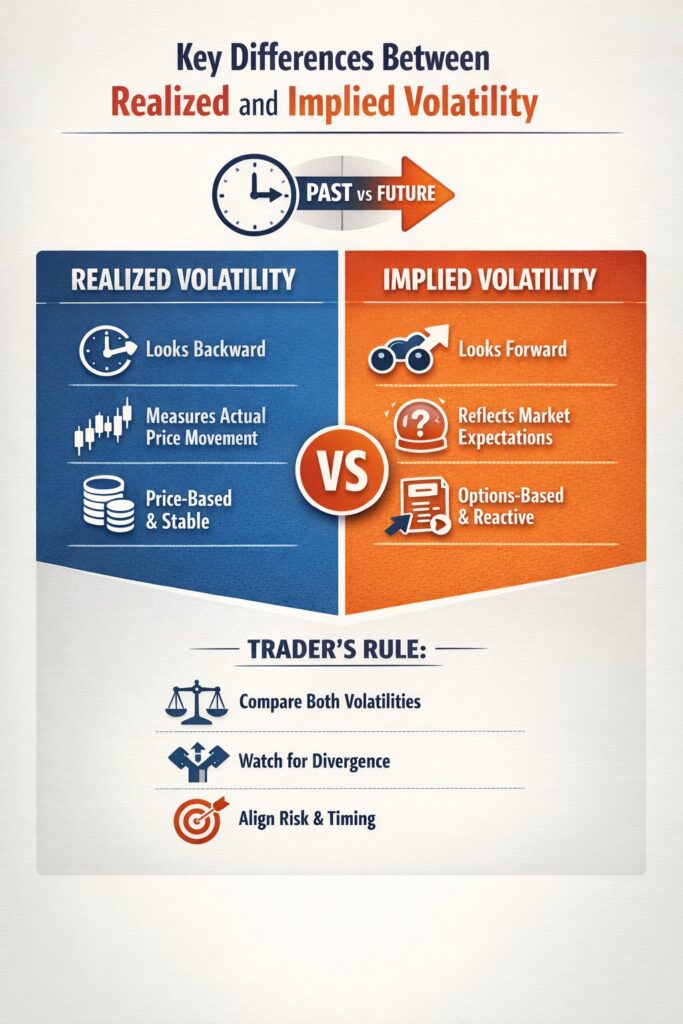
Key Differences Between Realised and Implied Volatility
The key difference between realised and implied volatility is time orientation.
Realised volatility looks backward and measures actual price movement. Implied volatility looks forward and reflects expectations.
Realised volatility is price-based, stable, and ideal for risk sizing. Implied volatility is options-based, reactive, and ideal for event risk and sentiment analysis.
Neither is sufficient alone. Effective Volatility Prediction comes from comparing both and understanding when they diverge.
Volatility Prediction Models in Quantitative Finance
Quantitative volatility models generally fall into two broad categories: traditional statistical models and hybrid models.
In practice, professional trading desks rarely rely on a single model. Instead, they compare model outputs to detect regime changes or abnormal risk conditions. When different models agree, confidence in the volatility forecast increases. When they diverge, it often signals a shift in market structure or the presence of event-driven risk.
Traditional Statistical Volatility Prediction Models
These models use historical prices and simple assumptions. They are popular because they are stable and interpretable. Common traditional statistical models are as follows:
- GARCH-family (adds persistence and mean reversion)
- Technical Indicators (Like ATR and EMWA)
Strength
- Clear logic, easy to implement, strong baseline for risk management
Weakness
- Mostly backwards-looking; reacts after volatility changes
GARCH Model for Volatility Prediction
The GARCH (Generalised Autoregressive Conditional Heteroskedasticity) model is a classical econometric approach for forecasting time-varying volatility in financial markets. As explained by Investopedia, GARCH is built on the idea that market volatility is conditional, meaning today’s risk depends on past information.
Unlike models that assume constant variance, GARCH recognises that financial returns show volatility clustering, where large price swings tend to be followed by more large swings, and small moves tend to persist during calm periods.
How the GARCH Volatility Prediction Model Works
Think of GARCH(1,1) as a clean recursion: it updates tomorrow’s volatility forecast using today’s information.
The GARCH model’s equations are as follows:
Return Equation: rt=μ + ɛt
Variance (Volatility) Equation: σt2=α0+α1 ɛ2t-1+β1 σ2t-1
- rt: The return of the asset at time t
- μ: The average or expected return
- ɛt: The shock or error term at time t
- σt: Conditional variance at time t (Variance)
- α0: constant term in the variance equation
- α1: Weight on recent shocks
- ɛ2t-1: Squared shock from the previous period
- β1: Weight on past volatility
- σ2t-1: Previous period’s variance forecast
In plain terms, GARCH says: today’s variance forecast is a weighted average of:
- A long-run average variance that the market tends to revert to,
- The previous predicted variance,
- The most recent shock, measured by the squared residual.
Recent shocks matter more because the model effectively gives more weight to recent data, akin to an exponentially weighted approach. This mechanism allows GARCH to capture realistic market behaviour.
Trading example
If a stock normally moves ~1% daily and prints a 4% move after earnings, GARCH increases forecast variance and gradually decays it rather than snapping back to 1%.
Key Points:
Higher-frequency approaches using intraday realised volatility can detect shocks earlier than GARCH, because they measure variability within the day using smaller intervals.
Strengths and Limitations of GARCH for Stock and Forex Volatility Prediction
According to Saltfinancial, the Basic GARCH(1,1) model has Strengths and Limitations that traders should pay attention to:
Strengths
- Captures persistence well in stocks and Forex
- Explainable, used widely in risk systems (VaR, margin, portfolio risk)
- Updates easily using the last forecast and the last shock
Limitations
- Basic GARCH(1,1) assumes symmetry (up and down shocks affect volatility equally)
- Real markets often show the leverage effect (down moves increase volatility more)
- Often built on daily closes, it can miss fast intraday shocks
- Intraday realised volatility can detect changes earlier
If you need asymmetry, you should use EGARCH or GJR-GARCH models.
Machine Learning Approaches to Volatility Prediction
Machine Learning (ML) is changing how traders analyse markets. Unlike standard tools, ML learns from historical data. It analyses thousands of past price movements to uncover hidden patterns.
According to Insightbig, models such as Random Forests, XGBoost, and Support Vector Machines (SVR) can capture nonlinearity, but performance depends on feature design, regime stability, and the validation method.
Understanding ML Algorithms
Random Forest works like a team of experts. It creates many decision trees. For example, to predict Gold volatility, an ML model may use features like:
- lagged returns
- volume
- VIX level
- macro calendar flags (CPI day vs normal day)
They average their results for a solid forecast.
XGBoost is even more advanced. It learns from its mistakes. If it predicts a low move for Bitcoin but the market crashes, it adjusts its internal weights to do better next time.
LSTM Volatility Prediction Models
A popular type of ML is the LSTM (Long Short-Term Memory) network. LSTMs are excellent for time-series data, such as Forex charts. They have a built-in “memory.” They remember events from the distant past.
For volatility prediction, an LSTM notices that Gold often drops after a sharp rise in December. It uses this memory to forecast future moves.
Numeric Example:
An LSTM model might analyse the last 50 days of EUR/USD data. It predicts that volatility will spike from 50 pips to 150 pips tomorrow. Traders use this to reduce size and widen stops.
Advantages and Challenges of Machine Learning Volatility Prediction
Using Machine Learning for volatility prediction changes how traders approach the market. It offers powerful tools but comes with specific risks. Below are the key benefits and drawbacks explained simply.
Advantages of Machine Learning
- Handles Complex Relationships: ML models such as Random Forests and XGBoosts handle non-linear patterns easily. They capture complex price-action curves that standard math misses.
- Uses Diverse Data Inputs: ML models can analyse multiple variables simultaneously. They look at lagged returns, trading volume, and macroeconomic news simultaneously. This gives a complete picture of why volatility is changing.
- Long-Term Memory: LSTM models act like a student that never forgets. They are excellent for time-series data.
- Self-Improvement: Models like XGBoost use “gradient boosting.” They learn from their mistakes. If the model predicts low volatility but the market crashes, it adjusts its internal weights to avoid repeating the same error.
Challenges of Machine Learning
- The “Black Box” Problem: One of the biggest issues is interpretability. ML models often provide predictions without explaining why. A chart might say “Sell,” but traders cannot easily see the logic behind the decision. This makes risk management harder.
- Risk of Overfitting: This occurs when a model memorizes past data rather than learning a general rule.
- High Complexity: Setting up these models requires coding skills in Python or R and significant computing power.
- Data Hunger: ML models need massive amounts of clean data. If the historical data has gaps or errors, the model’s predictions will be wrong.
Market Volatility Prediction Using Indicators
Indicators help traders spot volatility regimes (calm vs. expanding risk) using readily available market data. They don’t forecast exact volatility, but they improve trading decisions by guiding stop-loss, position, and strategy sizes.
The two most used tools are:
- price-based measures (Historical Volatility/ATR)
- and expectation-based measures (VIX).
Historical Volatility and ATR
Historical Volatility (HV) and Average True Range (ATR) are price-based indicators that measure an asset’s past price movements. Historical volatility is usually calculated as the standard deviation of returns over a fixed period, while ATR measures the average daily range, including gaps. Both are backwards-looking but extremely practical.
HV and ATR are simple, but they work because of volatility clusters. Their main weakness is their inability to anticipate events. They react only after price movement occurs, which is why they are often combined with forward-looking tools.
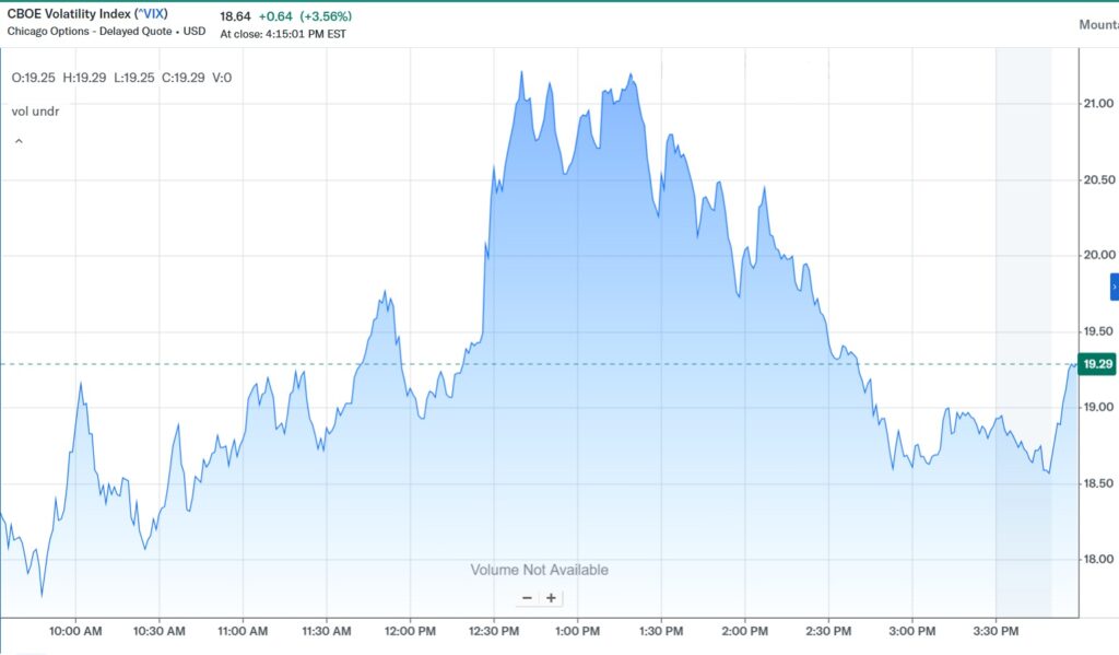
Volatility Index (VIX) and Market Expectations
Referring to quantified strategies, the Volatility Index (VIX) measures the market’s expected volatility over the next 30 days, derived from S&P 500 options prices.
VIX is forward-looking and reflects how much risk traders are pricing into the future. For this reason, it is often called the “fear index.”
- A VIX level around 12–15 indicates calm market conditions.
- A rise to 25–30 signals stress and expectation of large price swings.
- During crisis periods, the VIX can spike above 40, reflecting panic and extreme uncertainty.
Note:
Even traders who do not trade US indices watch VIX closely because it influences global risk sentiment, affecting Forex pairs, gold, and crypto markets.
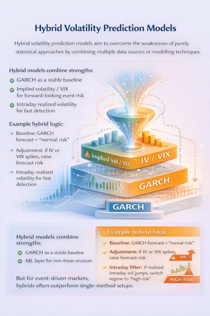
Hybrid Volatility Prediction Models
Hybrid volatility prediction models aim to overcome the weaknesses of purely statistical approaches by combining multiple data sources or modelling techniques.
Hybrid models combine strengths:
- GARCH as a stable baseline
- Implied volatility/VIX for forward-looking event risk
- Intraday realised volatility for fast detection
- ML layer for non-linear structure
Example hybrid logic
- Baseline: GARCH forecast = “normal risk”
- Adjustment: if IV or VIX spikes, raise forecast risk
- Intraday filter: if realised intraday vol jumps, switch regime to “high risk.”
The main trade-off is as follows:
- More complexity and maintenance
- Higher risk of overfitting if not controlled
- But for event-driven markets, hybrids often outperform single-method setups.
How to Predict Market Volatility
Predicting market volatility is about measuring the speed of price changes. Traders use a mix of tools to guess future movements. The main methods are statistical models, technical indicators, and market news analysis. The goal of volatility prediction is to estimate risk before placing a trade.
You can look at the past to see the future. Volatility regimes can shift after long compression, but timing is uncertain—use indicators like ATR expansion/Bollinger bandwidth rather than a named pattern.
How to Predict Market Volatility in Stock Markets
In the stock market, prediction relies heavily on the VIX and earnings reports. The VIX, or Fear Index, tracks expected volatility for the S&P 500. A rising VIX means traders are scared and expect big drops.
Earnings seasons are critical. Before a big company releases its profit numbers, volatility rises. Traders use options pricing to guess how much the stock will move.
Numeric Example: Imagine a stock like NVIDIA trades at $400. Before earnings, its options suggest it will move up or down by $20. This is a 5% expected move. If the report comes out and the price only moves $2, the volatility crushes, and the option price drops.
Predicting Volatility in the Foreign Exchange Market
Forex volatility is different because the market never sleeps. Here, the prediction concerns time and economics. The highest volatility happens when major trading sessions overlap. This is usually when London and New York are both open. Economic data releases, such as interest rate decisions or Non-Farm Payrolls (NFP), also cause massive spikes.
Numeric Example: On a quiet Tuesday, the EUR/USD pair might move just 30 pips per hour. However, during the US NFP release, it can move 150 pips in just one minute. Traders use economic calendars to predict these exact times.
Using Volatility to Predict Market Direction
Volatility does not directly predict direction, but it provides critical context for directional trades.
In practice, volatility indicates how reliable a price move is likely to be. Low-volatility environments usually favour range-bound behaviour, in which prices oscillate between clear support and resistance levels. High-volatility environments favour trend development or sharp reversals, as strong participation and risk-taking are common. Ignoring volatility often leads to false breakouts, premature entries, or oversized positions during unstable conditions.
For example, if a market breaks above resistance while volatility is expanding, the move is more likely to continue than during low volatility.
Note:
Traders use volatility as a confirmation filter: direction + volatility together provide stronger signals than price alone.
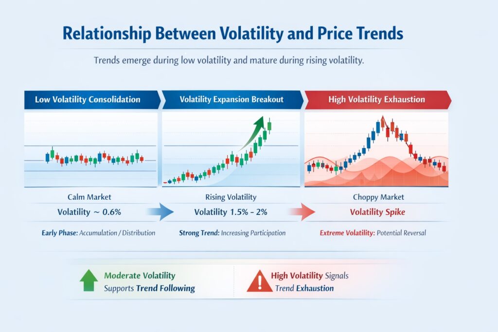
Relationship Between Volatility and Price Trends
A well-observed relationship exists between volatility and trends. Trends often emerge during periods of low volatility and mature during times of rising volatility.
Early trend phases typically show compressed volatility as accumulation or distribution occurs quietly. Once price breaks out, volatility expands as more participants enter the market.
For example, a stock consolidating with daily volatility near 0.6% may break out and quickly move to 1.5–2%, confirming trend strength.
However, extremely high volatility can signal trend exhaustion, especially near tops or bottoms, where panic buying or selling dominates.
For traders, this means that moderate volatility expansion supports trend-following strategies, while extreme volatility signals instability and potential reversals. Volatility, therefore, helps traders decide when to follow trends and when to reduce exposure, even if the direction still looks favourable on the chart.
Volatility Breakouts and Market Regime Shifts
Volatility breakouts often signal market regime shifts, where price behaviour changes structurally.
A regime shift occurs when a market moves from low volatility to high volatility, or from stable trends to chaotic movement. Volatility indicators like ATR expansion, Bollinger Band widening, or spikes in implied volatility help identify these transitions early.
Example:
If ATR on EUR/USD stays near 40 pips for weeks and suddenly jumps to 90 pips, the market has likely shifted from a range regime to a trending or news-driven regime. Strategies that worked before—tight stops, mean reversion—often fail after the shift.
Recognising volatility breakouts allows traders to adapt quickly by changing strategy, reducing leverage, or standing aside. In this sense, volatility is not just a risk metric; it is a signal of market structure.
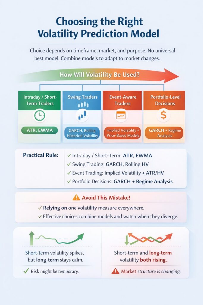
Best Volatility Prediction Models for Traders
The “best” volatility model is the one that matches your timeframe and decision (stop size, position size, or event risk). No single model wins in all markets. Use volatility models as risk tools, not direction signals.
In practice, traders use models to answer three questions:
- How wide should my stop be?
- How big should my position be?
- Is the market environment stable or unstable?
Based on this, the best volatility prediction could be as follows:
- Simple models such as ATR or EWMA often outperform complex models for short-term trading because they react quickly.
- More structured models, such as GARCH, are better for medium-term risk estimation.
- Long-term traders and investors focus less on day-to-day volatility and more on regime shifts and long-run variance.
Short-Term Volatility Prediction Models
Short-term volatility prediction focuses on immediate risk, usually from minutes to a few days. Models in this category must react fast and update easily. The most widely used tools are ATR, Historical Volatility, and EWMA. These models rely on recent price action and give traders a practical estimate of current market noise.
Short-term volatility models are fast and simple, which makes them ideal for trade execution and risk control. However, they react only after volatility rises, so they are weak at predicting upcoming events and should not be used for forecasting.
Long-Term Volatility Forecasting Approaches
Long-term volatility forecasting targets structural risk rather than daily fluctuations. These approaches are used by swing traders, portfolio managers, and risk desks. Common tools include GARCH-family models, long-horizon historical volatility, and regime-based analysis. The goal is to estimate how volatility behaves over weeks, months, or business cycles.
The limitation of long-term models is their lack of responsiveness. They are slow to adapt to sudden shocks and are not suitable for intraday decisions.
Their strength lies in strategic risk planning, not trade timing.
How to Convert Volatility into Stops and Position Size
Volatility is useless unless it changes your trade sizing.
Example
- Account: $10,000
- Risk per trade: 1% = $100
- EUR/USD stop: 80 pips
- Pip value (example): $1 per pip (micro/mini sizing varies)
Position size rule
- Size = Risk / (Stop × pip value)
- Size = 100 / (80 × 1) = 1.25 units of $1/pip exposure (adjust to lot type)
If ATR doubles, your stop usually widens. If stop widens, size must drop to keep risk fixed.
Conclusion
Volatility Prediction is a risk tool that estimates the size of future moves, not market direction. The practical edge is using it to adjust stop-loss distance, position size, and strategy choice as volatility regimes change. A simple workflow is: choose your timeframe, measure realised volatility, check forward-looking risk, select a matching model, and convert the output into clear risk rules.
The most reliable insight often comes from comparing realised and implied volatility—when they diverge, the market is warning you about changing conditions or event risk.