


Multi-factor models explain and forecast asset returns using multiple risk drivers, rather than just one, as in the CAPM. They include market, economic, and financial variables to give a more realistic view of risk and return.
As markets become more complex, understanding how these factors interact enables investors and analysts to make more informed decisions. This article covers the basics, key uses, and how multi-factor models improve investing and portfolio management.

- Multi-factor models help investors separate returns into market return, factor premia, and residual risk.
- A good multi-factor model reduces “unknown risk” by lowering the unexplained return (error term).
- Multi-factor models are useful for portfolio construction because they diversify across risk sources rather than just assets.
What are Multi-Factor Models in Finance?
According to Investopedia, a multi-factor model is a financial model that explains asset returns using multiple risk factors. Instead of relying on a single source of risk, the model assumes that several factors simultaneously drive price movements. These factors can be market-related, economic, or based on firm characteristics.
Purpose of Multi-Factor Models in Asset Return Analysis
The main purpose of a multi-factor model is to better explain why an asset earns a certain return. For example, a stock may rise not only because the overall market is rising, but also because it has small size or high value characteristics. By breaking returns into multiple drivers, investors can better understand risk and make better decisions.
Simple example:
If a stock returns 12% in one year, a multi-factor model may explain it as:
- 7% from market risk
- 3% from size factor
- 2% from value factor
This breakdown is not possible with a single-factor model.
Differences between single and multi-factor models in risk and return
A single-factor model, like CAPM, uses only one factor: market risk. It assumes that all returns depend mainly on market movements. This is simple, but often unrealistic.
Multi-factor models improve this by adding more factors. These models:
- Explain returns more accurately
- Capture different sources of risk
- Reduce unexplained return (error term)
Why do financial markets react to multiple risk factors?
Financial markets are complex. Prices react to:
- Interest rate changes
- Inflation
- Company size
- Value vs growth style
- Economic cycles
- and so on.
For example, during high inflation, value stocks may outperform growth stocks. A multi-factor model captures this Behaviour.
You can imagine returns like a layered diagram:
Market return at the base, style and economic factors on top, and asset-specific noise at the end.
This is why multi-factor models are widely used in modern finance.
The Role of Multi-Factor Models in Asset Pricing
A multi-factor model improves asset pricing by linking an asset’s expected return to multiple priced risk factors. Let’s see how.
How do multi-factor models impact asset pricing?
Multi-factor models enhance asset pricing by incorporating factors like size, value (book-to-market), interest rates, industry risk, and macroeconomic conditions. This provides a clearer understanding of the factors that drive an asset’s value, allowing investors to more accurately assess whether it is fairly priced.
Link between risk factors and expected returns
The link between risk factors and expected returns is one of the core insights provided by multi-factor models. The theory behind these models suggests that higher exposure to certain risk factors should be rewarded with higher expected returns. For example, stocks with higher value characteristics (such as low price-to-earnings ratios) or smaller market capitalisations often have higher expected returns because they are considered riskier.
Q: Why do small-cap stocks typically offer higher returns?
A: Small-cap stocks are considered riskier than large-cap stocks, so investors demand a higher return for taking on that risk. Multi-factor models capture this risk and can predict higher returns for small stocks over time.
Introduction to Risk Premia in Multi-Factor Models
In a multi-factor model, a risk premium is the extra return investors demand for bearing a specific type of risk. Each factor—such as market, size (small vs. large), or value vs. growth—has its own premium, and these premiums can differ across assets.
The model estimates an asset’s expected return by combining factor exposure with factor risk premiums.
Example: if the size premium is 4% and a stock has strong exposure to small-cap risk, investors expect an additional return of about 4% from that factor.
Risk premia matter because they tell you whether the return you expect is a fair payment for the risk you take.
CAPM vs Multi-Factor Models
The Capital Asset Pricing Model (CAPM) is the classic starting point for asset pricing. It gives a clean idea: the only risk that should earn an extra return is market risk, because other risks can be diversified away. Multi-factor models build on this idea by recognising the obvious truth that the CAPM ignores: markets price more than one kind of risk.
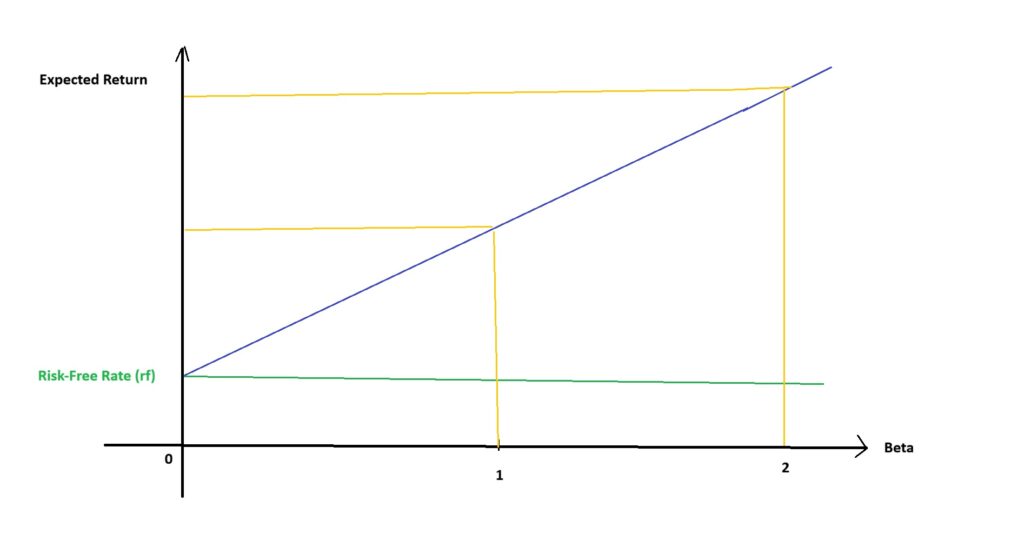
Overview and assumptions of CAPM
CAPM is a single-factor asset pricing model that estimates an asset’s expected return using just two inputs:
- the risk-free rate, and
- the asset’s market risk exposure (beta).
In simple terms, CAPM says:
- If a stock moves more than the market (i.e., has a high beta), investors demand a higher expected return.
- If it moves less than the market (low beta), the expected return should be lower.
CAPM is useful as a baseline—but often too simplistic for real-world return Behaviour.
Formula of CAPM
According to Wallstreetprep, the Camp formula is:
Ke = rf+β (rm-rf)
- Kf: Cost of equity (expected return on the asset)
- rf: Risk-free rate (the return on a risk-free asset, such as government bonds)
- β: Beta of the asset (a measure of how much the asset’s return moves in relation to the market)
- rm: Expected return of the market
- (rm-rf): Market risk premium (the extra return expected from the market over the risk-free rate)
The key idea is that investors require a higher return for taking on greater risk, as reflected in an asset’s beta.

Example:
If the risk-free rate (rf) is 3%, the expected market return (rm) is 8%, and the beta (β) of a stock is 1.5, the cost of equity (Ke) would be:
Ke = 3% + 1.5 × (8% – 3%)
Ke = 3% + 1.5 × 5% = 3% + 7.5% = 10.5%
This means that investors would expect a 10.5% return on this asset to compensate for the market risk.
Limitations of CAPM in real market returns
While CAPM provides a simple and elegant framework, its real-world applicability is often limited. One of the main criticisms is its assumption that only market risk affects an asset’s return. In reality, other factors such as interest rates, inflation, and company-specific risks can also play a significant role. For instance, a stock’s price may rise due to favourable changes in industry conditions rather than just market-wide movements.
Example:
During a market downturn, a tech stock might outperform the market if its earnings are strong, but CAPM wouldn’t capture this phenomenon.
Why do multi-factor models outperform CAPM?
Multi-factor models outperform the CAPM by accounting for a broader range of risk factors. These models account for factors such as company size, industry exposure, and macroeconomic variables, including interest rates and inflation. By incorporating multiple factors, these models provide more accurate predictions of an asset’s return, especially in complex, dynamic markets.
Why is CAPM still used as a base model?
Despite its limitations, CAPM remains a foundational concept in finance due to its simplicity and historical significance. It serves as an easy starting point for understanding the relationship between risk and return and is often used as a benchmark for comparing other models.
| Feature | CAPM (Single-Factor) | Multi-Factor Models |
|---|---|---|
| Primary Driver | Market Risk (Beta) only. | Multiple drivers (Size, Value, Momentum, Inflation, etc.). |
| Assumption | All other risks can be diversified away. | Specific risks (factors) earn specific premiums. |
| Accuracy | Lower (often leaves high unexplained error). | Higher (reduces the error term/residual). |
| Complexity | Low (Simple formula). | High (Requires extensive data and regression). |
| Best Use | Basic benchmarking & rough estimates. | Portfolio construction, risk management, & alpha generation. |

Key point
Investors may use CAPM to get a general sense of market risk before diving into more intricate multi-factor models that account for additional layers of risk.
Mathematical Structure of Multi-Factor Models
Multi-factor models use a mathematical framework to explain asset returns by considering multiple factors. Below is an explanation of the general structure and the role of each factor, along with an understanding of factor loadings and model errors.
General structure of Multi-Factor Models
The general structure of a multi-factor model is represented as:
Ri = α + β1F1 + β2F2 + … + βnFn + ε
Where:
- Ri = Return of the asset
- α = Intercept or constant term (often interpreted as the asset’s return when all factors are zero)
- β1, β2, …, βn = Factor loadings, representing the sensitivity of the asset to each factor
- F1, F2, …, Fn = Factors (e.g., market return, interest rates, company size, etc.)
- ε = Error term (residual return, unexplained by the factors)
This structure allows the asset return to be expressed as a linear combination of multiple factors, plus an error term representing the portion of the return that cannot be explained by the factors.
Role of each factor in returns
In a multi-factor model, each factor plays a specific role in explaining the asset’s return. For example:
- Market Factor: The overall market return (e.g., the S&P 500) often drives a significant portion of returns for most assets.
- Size Factor (SMB): Stocks of small-cap companies tend to have higher expected returns compared to large-cap stocks.
- Value Factor (HML): Stocks with low price-to-book ratios (value stocks) tend to outperform those with high price-to-book ratios (growth stocks).
- Other Factors: Depending on the model, these could include interest rates, inflation, or company-specific characteristics such as earnings growth.
Understanding factor loadings and model errors
Factor loadings (β coefficients) indicate the extent to which each factor influences the asset’s return. A high β value means that the asset is highly sensitive to changes in that factor.
For example, a high β1 (market factor) implies that the asset moves in close correlation with the overall market.
The error term (ε) represents the portion of the asset’s return that cannot be explained by the factors in the model. This could include unsystematic risks, company-specific events, or factors not included in the model.
Key point
The goal of the multi-factor model is to minimise the error term by carefully selecting the most relevant factors.
Example:
For a stock, if the market return (F1) is up by 5%, and the stock has a β1 of 1.2, then the expected return from the market factor would be 1.2 * 5% = 6%.
If other factors contribute an additional 3% and there’s an unexplained return of 1%, then the model’s error term would be 1%.
Types of Multi-Factor Models in Finance
According to CFA, multi-factor models in finance come in various forms, each serving different purposes in asset pricing and risk management.
Types of Multi-Factor Models are as follows:
| Model Type | Core Focus | Key Inputs | Famous Example |
|---|---|---|---|
| Macroeconomic | External economic forces. | GDP, Inflation, Interest Rates, Unemployment. | Chen, Roll, and Ross Model: Links returns to the industrial production and yield curve. |
| Fundamental | Company-specific traits. | P/E Ratio, Market Cap, Debt/Equity, Book Value. | Fama-French 3-Factor: Explains returns via Market, Size (SMB), and Value (HML). |
| Statistical | Mathematical patterns. | Historical price data (no economic theory required). | PCA (Principal Component Analysis): Identifies hidden correlations purely from data. |
Macroeconomic Factor Models
In macroeconomic factor models, the focus is on economic variables that affect asset returns. These factors can include GDP growth, inflation, interest rates, and unemployment rates.
A popular macroeconomic model is the Chen, Roll, and Ross (1986) model, which uses the following factors:
Ri = α + β1 * (Inflation) + β2 * (Interest Rates) + β3 * (Industrial Production) + β4 * (Yield Curve) + β5 * (Market Return)
Where:
- Ri = Asset return
- α = Intercept term
- β1, β2, β3, β4, β5 = Sensitivity of the asset to each macroeconomic factor
This model helps investors understand how economic factors, such as changes in inflation or interest rates, can affect asset prices.
Fundamental Factor Models
Fundamental factor models focus on company-specific factors, such as Price-to-Earnings (P/E) ratios, market capitalization, and financial leverage, to predict asset returns.
These models help assess a company’s intrinsic value and its stock performance.
For example, companies with high earnings growth or low debt often outperform others over time.
The Fama-French Model is a well-known fundamental factor model that has two versions:
Fama-French Three-Factor Model
The Fama-French three-factor model adds size and value factors to the traditional CAPM model to explain asset returns. It suggests small-cap stocks tend to outperform large-cap stocks, and value stocks (low price-to-book ratios) outperform growth stocks (high price-to-book ratios).
The formula for the Fama-French three-factor model is:
Ri = rf + β1 (rm – rf) + β2 (SMB) + β3 (HML)
Where:
- Ri = Asset return
- rf = Risk-free rate
- β1 = Market risk sensitivity (exposure to market returns)
- β2 = Sensitivity to the SMB factor (small minus big, size factor)
- β3 = Sensitivity to the HML factor (high minus low, value factor)
Fama-French Five-Factor Model
The Fama-French five-factor model extends the three-factor model by adding:
- RMW (Robust Minus Weak): Difference in returns between companies with strong vs. weak performance.
- CMA (Conservative Minus Aggressive): Difference in returns between companies with conservative vs. aggressive investment strategies.
The formula for the Fama-French five-factor model is:
Ri = rf + β1 (rm – rf) + β2 (SMB) + β3 (HML) + β4 (RMW) + β5 (CMA)
Statistical factor models
Statistical factor models use statistical techniques to identify hidden factors that affect asset returns. These models typically do not rely on predefined economic or company-specific factors but instead use methods such as Principal Component Analysis (PCA) or Factor Analysis to uncover the factors driving price movements.
A general form of a statistical factor model is:
Ri = α + Σ (βi * Fi) + ε
Where:
- Ri = Asset return
- α = Intercept term
- βi = Sensitivity to each identified factor
- Fi = Factor i (statistical component driving the return)
- ε = Error term (residual return not explained by the factors)
This model allows analysts to discover patterns and correlations in historical data and use them for forecasting asset returns.
A Simple Example of a Multi-Factor Model
To better understand how Multi-factor models work, let’s look at a simple conceptual example to explain their performance, interpret the outputs, and compare them with traditional single-factor models.
Conceptual example to explain model performance
Let’s consider a stock and use a basic multi-factor model to explain its return. Suppose the stock’s return is influenced by three factors:
- Market Risk (rm – rf)
- Size (SMB)
- Value (HML)
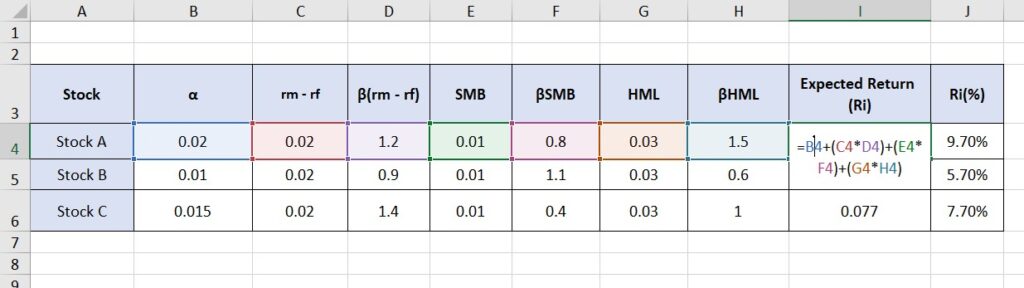
For this example, the model formula could look like this:
Ri = α + β1(rm – rf) + β2(SMB) + β3(HML) + ε
Now, let’s assume the following values:
- The market risk premium (rm – rf) is 5%.
- The size factor (SMB) is 2%.
- The value factor (HML) is 3%.
- The stock’s β values for each factor are:
- β1 = 1.2 (market)
- β2 = 0.8 (size)
- β3 = 1.5 (value)
The expected return for the stock would be calculated as follows:
Ri = α + (1.2 * 5%) + (0.8 * 2%) + (1.5 * 3%)
Ri = α + 6% + 1.6% + 4.5%
If the intercept (α) is 2%, the total expected return for the stock is:
Ri = 2% + 6% + 1.6% + 4.5% = 14.1%
Thus, the stock’s return is expected to be 14.1%, considering its exposure to market, size, and value factors.
Interpreting model outputs simply
To interpret the outputs of this multi-factor model:
- β1 (Market Risk): The stock moves 1.2 times more than the market. If the market rises by 5%, the stock is expected to rise by 6%.
- β2 (Size): The stock has a smaller sensitivity to size but still benefits from the small-cap premium, contributing 1.6% to its return.
- β3 (Value): The stock is more sensitive to value, contributing 4.5% to its return.
The error term (ε) represents any unexplained portion of the return.
Comparing single-factor vs multi-factor models
The CAPM model only considers market risk and calculates the return as:
Ri = rf + β1(rm – rf)
For β1 = 1.2 and a 5% market risk premium:
CAPM: Ri = rf + 6%
In contrast, the multi-factor model considers market, size, and value factors, providing a return of 14.1%. The multi-factor model offers a more comprehensive view of asset returns, whereas the CAPM focuses solely on market risk, ignoring factors such as size and value.
Multi-Factor Models in Portfolio Management
Multi-factor models help portfolio managers understand where returns and risks actually come from. Instead of looking only at assets, these models analyse factor exposures such as market, value, size, momentum, and interest rates. This approach makes portfolio decisions more transparent and controllable.
Measuring Factor Exposures (Portfolio Diagnostics)
The first step in factor-based portfolio management is diagnostics. Multi-factor models measure how sensitive each asset—and the portfolio as a whole—is to different risk factors.
For example, a portfolio may appear diversified across many stocks but still have:
- High exposure to growth stocks
- Strong sensitivity to interest rates
- Hidden concentration in market risk
Factor diagnostics reveal these hidden exposures and show what truly drives portfolio performance.
Managing Risk with Factor Exposure Control
Once factor exposures are identified, managers can actively control risk. Instead of selling entire positions, they can adjust exposure at the factor level.
Common actions include:
- Reducing market beta during high-risk periods
- Lowering interest-rate exposure when rates are volatile
- Hedging unwanted factor risk using derivatives or offsets
This approach allows for more precise risk management than traditional asset-only methods.
Factor-Based Diversification (Avoiding Hidden Concentration)
True diversification means spreading risk across different factor premia, not just holding many assets.
A portfolio can hold dozens of securities and still be overexposed to one factor, such as growth or momentum. Multi-factor models help managers:
- Balance exposure between value and growth
- Combine defensive and cyclical factors
- Reduce hidden concentration risk
This leads to better risk-adjusted returns over time.
Factor-Based Portfolio Optimisation
Factor-based optimisation improves traditional portfolio construction by optimising factor exposures rather than relying solely on historical returns and correlations. The goal is to build portfolios that remain stable across different market regimes.
Setting Factor Targets and Computing Weights
In factor-based optimisation, managers define target factor exposures (for example, a neutral market beta, positive value exposure, and low interest-rate sensitivity). Portfolio weights are then calculated to match these targets as closely as possible.
Factor-Based vs Mean-Variance Optimisation
Traditional mean-variance optimisation relies on historical returns and correlations, which are often unstable and noisy. Factor-based optimisation focuses on economic drivers of risk and return.
As a result, factor-based portfolios are usually:
- More robust across market cycles
- Easier to explain and monitor
- Less sensitive to estimation errors
This makes factor-based optimisation better suited for long-term, professional portfolio management.
Summary Table (Portfolio Management and Factor Optimisation)
| Topic | What It Does | Why It Helps | Practical Example |
|---|---|---|---|
| Factor diagnostics | Measures portfolio exposure to factors (betas) | Finds hidden concentration risk | Portfolio holds 30 stocks but is still “all growth.” |
| Factor risk control | Adjusts exposure via rebalance/hedge/offset | Reduces risk at the source | Cut interest-rate sensitivity when rate volatility rises |
| Factor diversification | Spreads risk across different factor premia | Improves risk-adjusted returns | Combine value + quality + low-vol instead of only momentum |
| Factor-based optimization | Sets target factor exposures and solves for weights | Creates stable, explainable portfolios | Target beta ≈ 1, value tilt, low rate exposure |
| Mean-variance (traditional) | Optimises using historical returns/correlations | Can be unstable due to noisy inputs | Weights swing wildly when correlations shift |
Multi-Factor Models in Stock Selection
Multi-factor models are widely used in stock selection to identify stocks with better risk-adjusted return potential. This approach is especially popular in systematic and quantitative investing, where decisions are data-driven and rules-based.
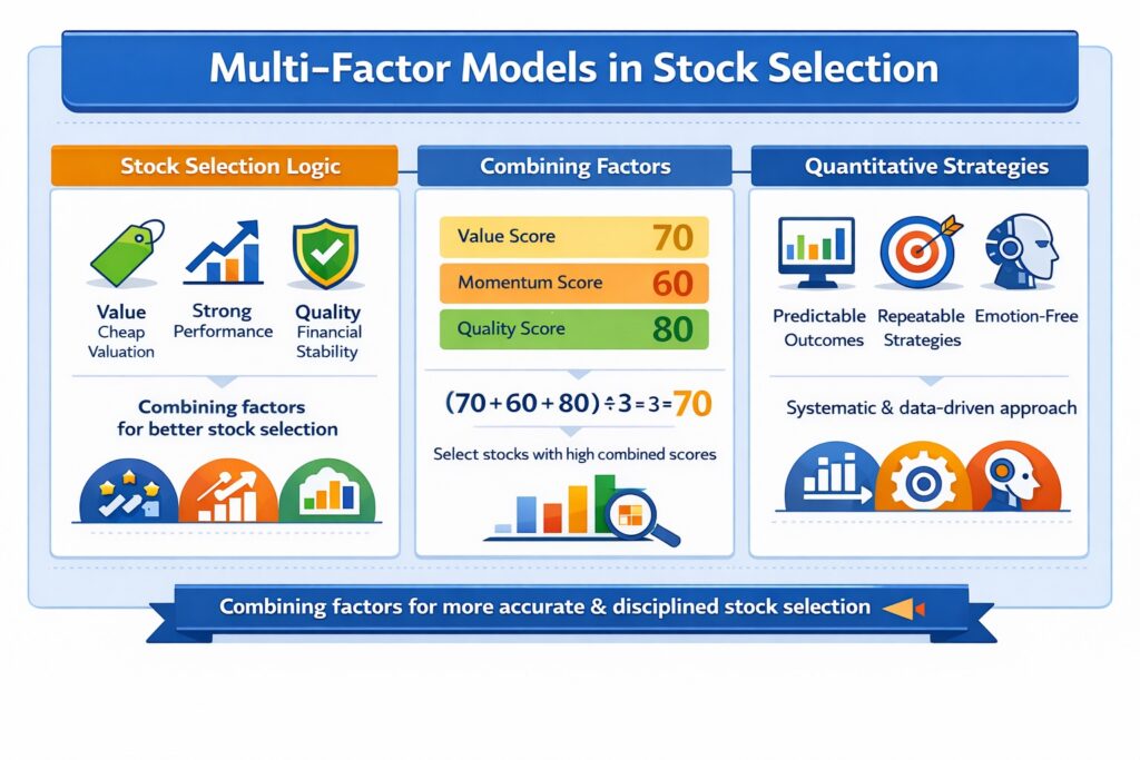
Logic behind multi-factor stock selection models
The core logic of multi-factor stock selection is simple:
Stocks that score well on several proven factors tend to outperform over time.
Each factor represents a source of return or risk, such as value, momentum, size, or quality.
For example, a stock may be attractive because it is:
- Cheap (value factor)
- Showing strong recent performance (momentum factor)
- Financially stable (quality factor)
Combining factors to create investment signals
Investment signals are generated by combining multiple factor scores into a single final score. Each factor is usually standardised and weighted.
Simple example:
- Value score = 70
- Momentum score = 60
- Quality score = 80
If all factors are equally weighted, the combined score is:
(70 + 60 + 80) / 3 = 70
Stocks with higher combined scores are selected for the portfolio.
This method helps avoid false signals that may appear when using only one factor.
Q: Why not use just one strong factor?
A: Single factors can underperform for long periods. Combining factors improves consistency.
Role in quantitative investment strategies
Multi-factor stock selection is a core component of quantitative (quant) strategies. These strategies rely on rules, data, and models instead of subjective judgment.
In quant investing:
- Factors are tested historically
- Signals are generated automatically
- Portfolios are rebalanced regularly
Multi-factor models allow quant strategies to be scalable, repeatable, and emotion-free.
This is why many ETFs, hedge funds, and algorithmic strategies are built on multi-factor stock selection models.
Implementing Multi-Factor Models with Python or Excel
Implementing multi-factor models is essential for analysing asset returns and managing investment portfolios. While both Python and Excel can be used to build these models, the choice of tool depends on the complexity, scale, and automation required.
Below are the implementation steps, the differences between Python and Excel, and the importance of data quality and timing in the process.
Steps for implementing multi-factor models
- Data Collection: Gather historical data for the factors (e.g., market return, size, value) and asset returns. This data can be sourced from financial databases such as Bloomberg Terminal and Yahoo Finance, or from publicly available datasets.
- Factor Selection: Choose the factors that you believe will explain the asset’s return (e.g., market risk, size, value, momentum).
- Calculate Factor Exposures: Use regression analysis to calculate the factor loadings (β coefficients).
- Combine Factors: Once you have the factor loadings, combine the individual factors to calculate the expected return using the multi-factor model formula.
- Optimisation: After calculating the expected returns for all assets, use portfolio optimisation techniques to allocate assets efficiently, balancing return and risk.
- Backtesting: Test the model using historical data to assess how well it predicts returns. Adjust and optimise the model as necessary.
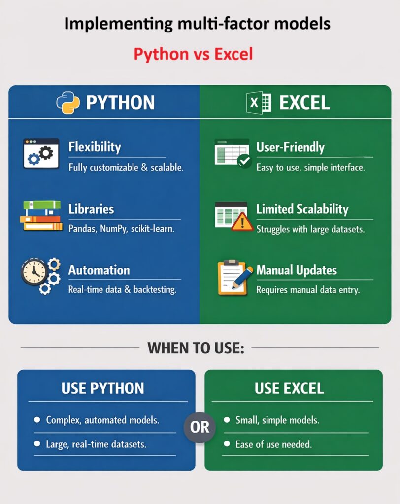
Differences between Python and Excel for implementation
- Python:
- Flexibility: Python allows for full customisation and automation. It is ideal for complex models with large datasets and can handle multiple factors with ease.
- Libraries: Python has powerful libraries like pandas, numpy, statsmodels, and scikit-learn for data manipulation, regression analysis, and machine learning.
- Automation: Python scripts can be automated for real-time data fetching and backtesting, making them suitable for more advanced implementations.
- Excel:
- User-Friendly: Excel is widely used for its simplicity and ease of use, making it suitable for less complex models and smaller datasets.
- Limited Scalability: While Excel offers basic functions for regression analysis and data manipulation, it struggles with large datasets and automation.
- Manual Updates: Data collection and model updates in Excel require manual input, making it less efficient for continuous monitoring.
When to Use:
- Use Python for scalable, automated, and data-intensive models.
- Use Excel for smaller datasets and simpler models, especially when ease of use is a priority.
Importance of quality data and timing
A multi-factor model is only as good as the data feeding it and the timing of your analysis.
- Quality matters: If your data is inaccurate, outdated, or too short in history, your factor results get distorted, and your decisions become garbage. Use reliable sources and enough time coverage to capture real trends.
- Timing matters: Real-time (or near real-time) data improves signals. Delayed data can break the model, especially in volatile markets. Even with historical models, you must account for current market conditions and regime changes.
Limitations and Risks of Multi-Factor Models
Multi-factor models are powerful, but they are not magic. Many investors misuse them by treating models as guarantees instead of tools. Understanding their limitations is critical if you want to use them professionally and avoid false confidence.
Risks of overfitting when selecting factors
Overfitting occurs when a model is trained to perfectly fit past data but fails to generalise to new data. This often occurs when too many factors are added or when factors are chosen only because they worked historically.
Example:
A model with 10 factors may look amazing in backtests, but once market conditions change, most of those factors stop working. The result is strong historical performance and weak real-world results.
Instability of factors over time
Factors are not stable forever. A factor that works well in one decade may underperform or disappear in another.
For example:
- Value factors can underperform during long growth-driven markets.
- Momentum factors can fail during sharp market reversals.
Economic regimes change, central bank policies shift, and investor Behaviour evolves. Multi-factor models must be reviewed and updated, not blindly reused.
Performance variation across markets
A factor that works in one market may fail in another.
Examples:
- Size and value factors work well in developed equity markets but may behave differently in emerging markets.
- Crypto markets often react more to liquidity and sentiment than to traditional value factors.
Multi-factor models must be market-specific. Copy-pasting a model from U.S. equities into forex or crypto is lazy and risky.
Why multi-factor models don’t guarantee profits
Multi-factor models explain expected returns, not guaranteed outcomes. Markets are influenced by:
- Black swan events
- Policy shocks
- Behavioral biases
Even a well-built model can underperform for long periods. That does not mean the model is broken—it means risk still exists.
Multi-factor models improve decision-making, not certainty. If you expect guaranteed profits, you’re using the wrong tool.
Impact of Multi-Factor Models on Risk and Return in Different Market Conditions
Multi-factor models do not behave the same in every market regime. If you ignore market conditions, your model results can look “wrong” even when the math is fine. The real issue is that factor premia are regime-dependent.
Performance in bullish vs bearish markets
In bull markets, risk-on factors often dominate:
- Momentum can perform well because trends persist.
- Growth can beat value when liquidity is strong.
- Small-cap (SMB) stocks may outperform if investors seek higher risk.
In bear markets, defensive Behaviour often changes factor returns:
- Quality (low debt, stable earnings) tends to hold up better.
- Low volatility factors can outperform by losing less.
- Value may or may not help—during deep risk-off phases, cheap stocks can stay cheap.
Effects during market volatility or financial crises
During crises, relationships break. Correlations rise, liquidity dries up, and models become less stable. Two common problems:
- Factor crowding: too many investors hold the same factor trades, causing forced selling.
- Rapid regime shifts: yesterday’s winning factor becomes tomorrow’s loser.
Example:
A momentum portfolio may crash in a “trend reversal” week because winners become losers fast.
In crises, your model’s error term (ε) often grows. That means more return is unexplained, so confidence should go down.
Comparing model effectiveness in high vs low volatility
In low volatility environments:
- Factor signals tend to be cleaner.
- Trends last longer.
- Multi-factor models often show stronger consistency.
In high volatility environments:
- Noise increases.
- Factor returns become unstable.
- Short-term performance becomes harder to predict.
Practical takeaway:
If volatility spikes, reduce leverage, widen risk limits, and rely more on robust factors (quality/low vol) instead of fragile ones (pure momentum).
Best Practices for Professional Use of Multi-Factor Models
Using multi-factor models professionally means treating them as structured decision tools, not as prediction machines. The difference between amateurs and professionals is not the model itself, but how it is used, tested, and controlled.
Selecting factors based on evidence
Choose factors backed by academic research and long-term empirical evidence, not recent performance or hype. A factor should:
- Work across long time periods
- Be economically explainable
- Survive different market cycles
If you can’t explain why a factor should earn a premium, you probably shouldn’t use it.
Out-of-sample testing
Never trust a model tested only on historical (in-sample) data. Always use out-of-sample testing to see how the model performs on unseen data.
Example:
- Build the model using 2000–2015 data
- Test it on 2016–2024 data
If performance collapses out-of-sample, the model was overfit.
Combining factor analysis with human judgment
Models don’t understand context. Humans do.
Factor models should be adjusted when:
- Market regimes change
- Structural events occur (rate shocks, regulations, crises)
- Data quality deteriorates
Use judgment to override or scale exposure, not to randomly interfere.
Table: Best Practices for Professional Use of Multi-Factor Models
| Best Practice | What to Do | Why It Matters |
|---|---|---|
| Select factors based on evidence | Use factors supported by strong research, a long history, and a clear economic reason | Prevents chasing hype and reduces weak/false factors |
| Out-of-sample testing | Build on one period, test on a different unseen period (e.g., train 2000–2015, test 2016–2024) | Detects overfitting and shows real-world robustness |
| Combine with human judgment | Adjust exposures when regimes change, crises happen, or data quality drops | Models miss context; judgment prevents blind mistakes |
| Use models as decision tools | Use models to rank, manage exposure, and stay consistent—not to “predict perfectly” | Keeps expectations realistic and improves decision quality |
Conclusion
Multi-factor models give a clearer picture of why assets move by linking returns to multiple risk drivers (market, size, value, macro factors, etc.). They are useful for asset pricing, portfolio management, optimisation, and stock selection, but they can fail if you use bad data, overfit factors, or ignore changing market regimes. Used correctly—with testing and discipline—they improve decisions. Used blindly, they produce confident mistakes.