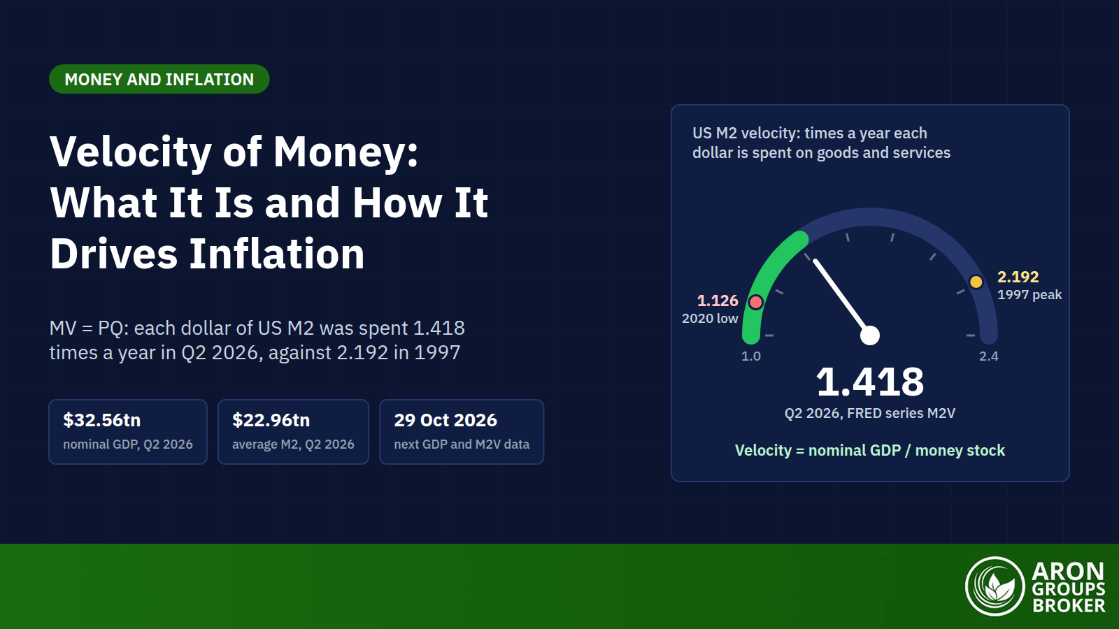

The velocity of money is how fast money circulates in an economy. It counts how many times each unit of currency is spent on goods and services in a given period. A dollar that is spent, re-spent and spent again has high velocity, while a dollar that sits in a savings account has low velocity.
It matters again because velocity has turned up while inflation runs above the Fed’s 2% goal. FRED data updated on 30 September 2026 put US M2 velocity at 1.418 for the second quarter, the highest since the end of 2019. On 14 October the Bureau of Labor Statistics (BLS) reported inflation of 3.7% in the year to September. The Fed had already raised the federal funds rate target range to 3.75% to 4.00% on 16 September.
This guide works through the formula with FRED data, the quantity theory behind it and the long fall in velocity. It then explains why quantitative easing did not cause runaway inflation, what happened in 2021 and what velocity means for traders.
- The velocity of money equals nominal GDP divided by the money supply. It comes from the equation of exchange, MV = PQ, which holds by construction.
- In Q2 2026 US nominal GDP ran at $32.56 trillion a year and M2 averaged $22.96 trillion. That is a velocity of 1.418 on FRED data updated on 30 September 2026.
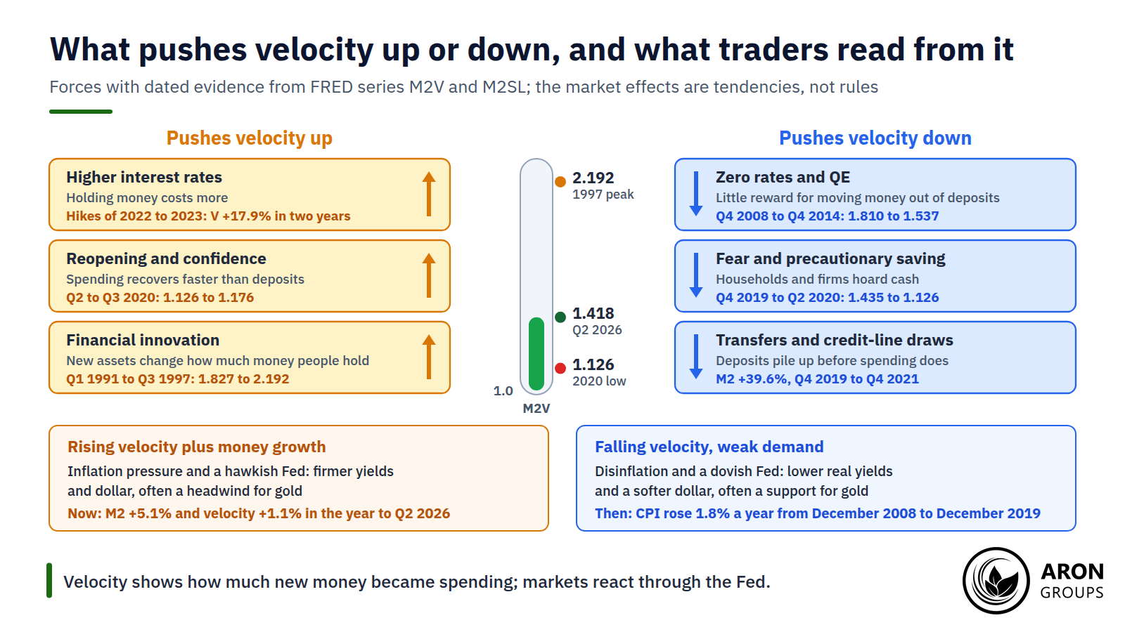
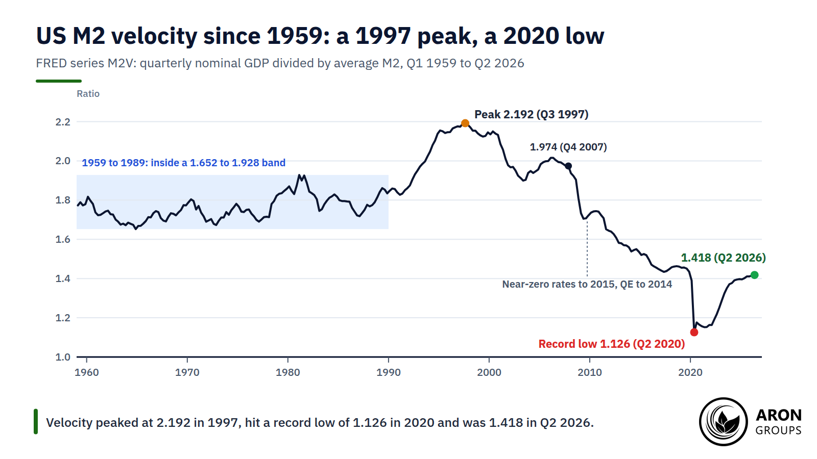
- M2 velocity peaked at 2.192 in Q3 1997 and fell 48.6% to a record low of 1.126 in Q2 2020, before recovering to 1.418.
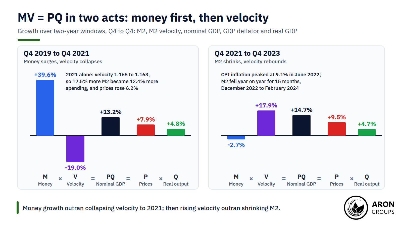
- Velocity did not rebound in 2021: it ended the year at 1.163 against 1.165. The rebound came from Q4 2021 to Q4 2023, when it rose 17.9% while M2 shrank 2.7%.
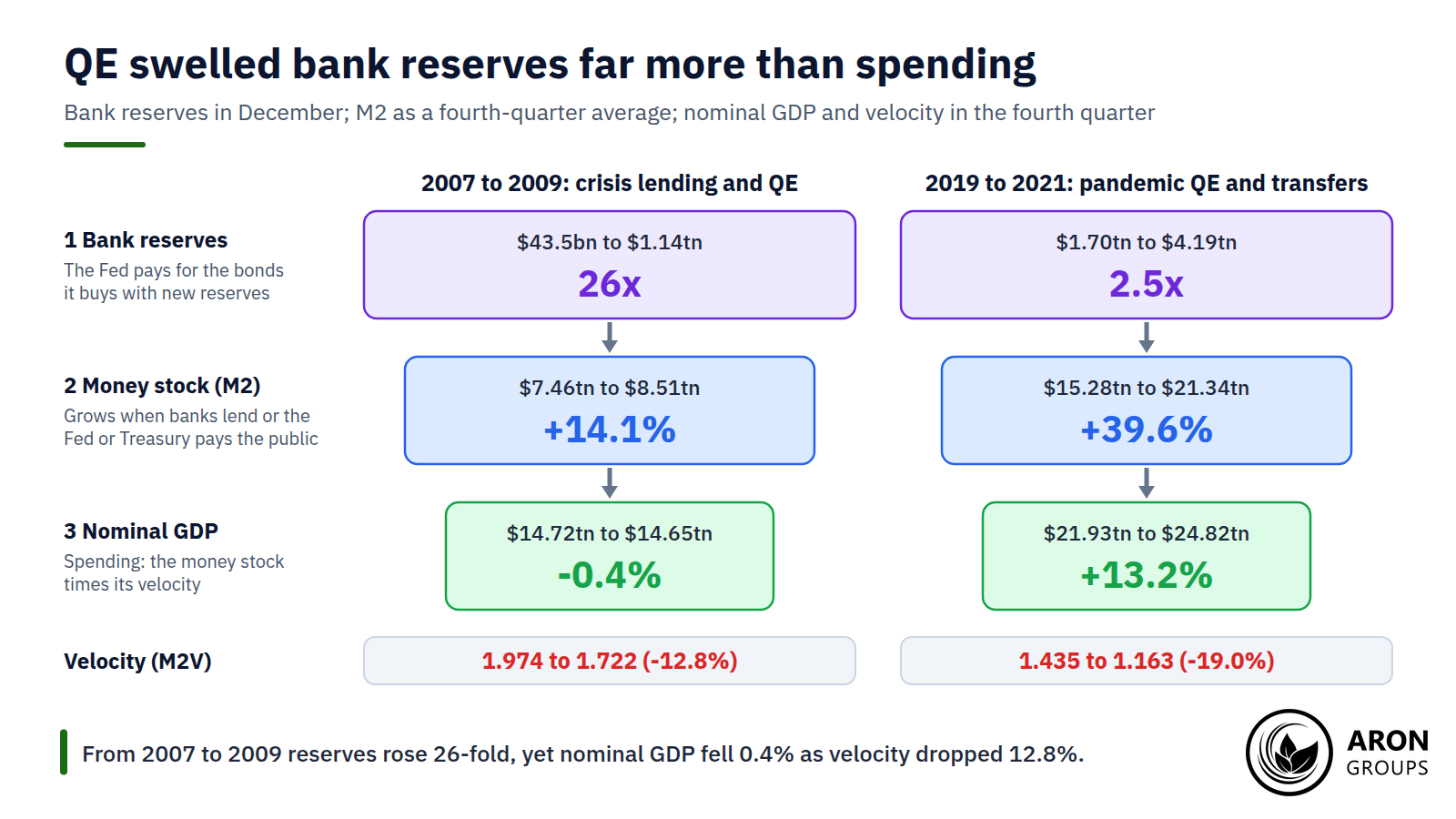
- Bank reserves rose 26-fold from December 2007 to December 2009. Yet from Q4 2007 to Q4 2009, M2 grew 14.1%, nominal GDP fell 0.4% and velocity dropped 12.8%.
What Is the Velocity of Money?
The velocity of money measures how many times, on average, each dollar is spent on newly produced goods and services over a year. FRED, the St. Louis Fed’s database, gives a velocity of money definition: the number of times one dollar is spent per unit of time. It is a rate of turnover, not an amount of money.
Risk Disclosure
Trading forex and CFDs carries a high level of risk and can result in the loss of all your capital. This content is educational and is not investment advice. Never risk money you cannot afford to lose.
High Velocity vs Low Velocity
High velocity means money is changing hands quickly. Households and firms spend what they receive, which signals an active economy, and it can push prices up when output cannot keep pace. US M2 velocity peaked at 2.192 in Q3 1997, during the long expansion of the 1990s.
Low velocity means money is being saved or hoarded rather than spent. That often signals weak demand, uncertainty or recession, though near-zero interest rates also hold it down. In a deep slump it can come with deflation: US consumer prices fell 1.4% in the year to June 2009, led by energy. In the 2020 lockdowns, M2 velocity fell 21.5% in two quarters.
Which Money? M1, M2 and the 2020 Break
Velocity can be measured against any money aggregate. In the Fed’s definitions, M1 is currency plus transaction deposits, while M2 adds small time deposits and retail money market funds. M2 is the usual choice for velocity work, partly because M1 has a break.
The Fed scrapped its six-transfers-a-month savings limit in April 2020. A February 2021 revision of its H.6 money data moved savings deposits into M1 from May 2020, lifting M1 sharply but leaving M2 unchanged. FRED’s M1 velocity drops from about 5.3 to about 1.3 between the first and third quarters of 2020. Comparisons of M1 velocity across 2020 are therefore misleading.
The Velocity of Money Formula and the Equation of Exchange
The velocity of money formula comes from the equation of exchange, MV = PQ. M is the money supply, V is velocity, P is the price level and Q is real output. P multiplied by Q is nominal GDP, the value of everything produced at current prices.
Rearranged, MV = PQ gives the velocity of money equation, V = PQ / M: nominal GDP divided by the money supply. FRED calculates it each quarter as nominal GDP at an annual rate, divided by the average of M2 over the quarter’s three months.
Irving Fisher popularised the equation in The Purchasing Power of Money in 1911. He wrote it as MV + M’V’ = PT, giving bank deposits their own velocity and using T for the total volume of trade. Modern versions use GDP, which statisticians measure every quarter.
Mini Example: How to Calculate the Velocity of Money for Q2 2026
Step 1: take nominal GDP. The Bureau of Economic Analysis (BEA) put second-quarter GDP at an annual rate of $32,563.0 billion in its 30 September third estimate.
Step 2: average the money stock. M2 was $22,756.6 billion in April, $23,013.7 billion in May and $23,114.9 billion in June, an average of $22,961.7 billion.
Step 3: divide. $32,563.0 billion divided by $22,961.7 billion gives 1.418, matching FRED’s published figure. Each dollar of M2 supported about $1.42 of annual spending on final output.
The same identity works as a simple velocity of money calculator. If M2 grows 5% in a year and velocity holds steady, nominal GDP also grows 5%. If real output then grows 2%, prices must rise about 2.9%, because 1.05 divided by 1.02 is 1.029.
The Long Decline and Partial Rebound of US Money Velocity
US M2 velocity has not simply declined for decades. From 1959 to 1989 it moved inside a band of 1.652 to 1.928. It peaked at 2.192 in Q3 1997, then fell for more than two decades to a record low of 1.126 in Q2 2020.
Since then it has recovered to 1.418, 25.9% above the low but still 35.3% below the 1997 peak. The sharpest drops came in recessions: 13.6% between Q4 2007 and Q2 2009, and 21.5% in the first half of 2020.
Why Velocity Fell
Velocity is a residual, whatever nominal GDP divided by M2 happens to be, but it moves for economic reasons. A central one is the opportunity cost of holding money, which vanishes when rates are near zero. The effective fed funds rate averaged between 0.07% and 0.24% in every month from December 2008 to December 2015.
Fed Board staff found a stable relationship between M2 velocity and that opportunity cost until the late 1980s. In the early 1990s velocity rose further than rates could explain. A 2015 Dallas Fed working paper added risk premia, financial innovation and banking regulation as major influences since 1929.
Payment technology is hard to measure. Faster digital payments can reduce the cash people need for transactions, which should lift velocity. M2 also holds savings and money market fund balances, so the effect on this measure is hard to isolate.
Velocity and the Quantity Theory of Money
Velocity is the key variable in the quantity theory of money. Together, money times velocity equals nominal spending; inflation is the part of its growth that real output does not absorb. If V were constant and Q grew at its normal pace, every extra point of money growth would show up one for one in prices. The catch is that velocity is not constant.
Key Point
MV = PQ always holds, because velocity is defined as nominal GDP divided by money. The quantity theory adds a testable claim: that velocity is stable, so money growth sets inflation.
Monetarists, led by Milton Friedman, treated velocity as stable enough for money growth to guide the Fed. In A Monetary History of the United States (1963), he and Anna Schwartz called poor Fed policy the primary cause of the Great Depression.
John Maynard Keynes had challenged that view decades earlier. His liquidity preference theory, set out in The General Theory in 1936, made the demand for money depend on interest rates. That implies velocity rises and falls with rates rather than holding steady.
The data sided with the sceptics for a generation. An IMF explainer notes that velocity became highly unstable in the 1980s and 1990s. The link between money and nominal GDP broke down, which most economists blame mainly on banking rule changes and financial innovation.
Quantitative Easing, Bank Reserves and the Missing Inflation
Quantitative easing shows why money creation and inflation can drift apart. When the Fed buys bonds, it pays with new bank reserves: balances that banks hold at the Fed and that households cannot spend. Reserves are the base layer of dollar liquidity, not money in your pocket.
M2 grows mainly when new money reaches the public: when banks lend, when the Fed buys from non-banks or when the Treasury pays people. From December 2007 to December 2009, crisis lending and asset purchases lifted total reserves 26-fold, from $43.5 billion to $1.14 trillion.
Yet between the fourth quarters of 2007 and 2009, M2 grew just 14.1% and nominal GDP fell 0.4%, so measured velocity dropped 12.8%. Rates then stayed near zero for seven years, and consumer prices rose just 1.8% a year on average from December 2008 to December 2019.
Why 2020 Was Different
In the pandemic, the new money did reach the public. Reserves rose about 2.5 times from December 2019 to December 2021, but this time M2 also jumped 39.6% from Q4 2019 to Q4 2021. Stimulus payments, business loans and credit-line draws all landed in bank accounts.
A June 2022 Fed Board note named four drivers of that deposit growth: credit-line drawdowns, Fed asset purchases, fiscal stimulus and a higher saving rate. Unlike reserves, money that households hold in deposits can be spent later.
Why the 2021 Inflation Was Different
A popular story says velocity rebounded in 2021 and unleashed inflation. FRED’s data do not support it. Velocity did bounce from 1.126 to 1.176 in Q3 2020 as the economy reopened. Through 2021 it hovered near 1.16, ending the year at 1.163 against 1.165 a year earlier: it stopped falling rather than rebounding.
What changed was that falling velocity stopped absorbing money growth. In 2020, M2 rose 24.1% but velocity fell 18.8%, so nominal GDP grew only 0.7%. In 2021, M2 rose another 12.5% with velocity flat, and nominal GDP jumped 12.4%.
The table splits each year’s growth in nominal GDP into money and velocity on one side, and prices and real output on the other. Growth rates multiply rather than add: for 2020, 1.241 × 0.812 = 1.007.
| Year | Money, M2 (M) | Velocity (V) | Nominal GDP (PQ) | GDP deflator (P) | Real GDP (Q) | CPI, Dec to Dec |
|---|---|---|---|---|---|---|
| 2019 | +6.8% | -1.8% | +4.9% | +1.5% | +3.4% | +2.3% |
| 2020 | +24.1% | -18.8% | +0.7% | +1.6% | -0.9% | +1.4% |
| 2021 | +12.5% | -0.2% | +12.4% | +6.2% | +5.8% | +7.0% |
| 2022 | +0.2% | +7.7% | +7.9% | +6.5% | +1.2% | +6.5% |
| 2023 | -3.0% | +9.5% | +6.3% | +2.8% | +3.4% | +3.4% |
| 2024 | +3.2% | +1.9% | +5.1% | +2.4% | +2.6% | +2.9% |
| 2025 | +4.1% | +1.0% | +5.1% | +3.0% | +2.0% | +2.7% |
MV = PQ, fourth quarter on fourth quarter, % change, rounded. Sources: FRED series M2SL, M2V, GDP and GDPC1; CPI from the BLS.
Then the roles swapped. From Q4 2021 to Q4 2023, M2 shrank 2.7% while velocity rose 17.9%, so nominal spending still grew 14.7%. M2 fell year on year from December 2022 to February 2024, which the St. Louis Fed says had not happened in any month since at least 1959.
CPI inflation peaked at 9.1% in June 2022, the largest 12-month rise since November 1981. Higher rates then raised the cost of holding money. The Fed began hiking in March 2022 and reached a target range of 5.25% to 5.50% in July 2023.
Research backs this money-first reading of the surge. A January 2023 BIS Bulletin found the money-inflation link close to one for one in high-inflation periods and almost absent in low-inflation ones. In the recent surge, countries with stronger money growth saw markedly higher inflation.
Q: Did money printing cause the 2021 to 2022 inflation?
A: It was a major ingredient, not the only one. M2 grew 39.6% in the two years to Q4 2021, and once velocity stopped falling that money reached spending. Reopening demand and supply shocks added to the pressure, and a St. Louis Fed economist argued in March 2025 that pandemic deficits were the primary driver.
Why Velocity Matters for Traders: Inflation, the Fed, Gold and the Dollar
Velocity matters to traders through one chain: money times velocity equals nominal spending, spending feeds inflation, and inflation shapes Fed policy. Policy in turn can move currencies, gold and bond yields. ESMA has warned that some retail investors do not fully appreciate the link between inflation and financial markets.
Rising velocity plus money growth points to inflation pressure and tighter policy, which tends to lift yields and the dollar. Falling velocity points to weak demand and a dovish Fed. Lower real yields, meaning interest rates after inflation, have often supported gold, which pays no interest.
Reading the Current Regime
In the year to Q2 2026, M2 grew 5.1% and velocity 1.1%, so nominal GDP rose 6.3%. That split into 2.2% real growth and 4.0% higher prices on the GDP deflator. September CPI was 3.7%, but core inflation was 2.6%: energy, up 20.4%, accounts for most of the gap.
The Fed’s 16 September statement called inflation elevated and growth solid. Markets will now scrutinise the 27 to 28 October meeting and the December dot plot. Velocity is quarterly and revised, so treat it as a slow regime lens, not a trading signal. Check it against CPI releases and Treasury yields.
The Honest Limits of the Velocity of Money
MV = PQ always holds, so it cannot prove causation. Velocity is a residual, so any error in GDP or in the money data flows straight into it. The equation cannot say whether money pushed prices or prices pulled money.
The choice of money matters too. M2 includes retail money market funds, which, as an investor.gov guide explains, pay dividends that generally reflect short-term interest rates. When savers move into Treasury bills or institutional funds outside M2, measured velocity rises even if spending is unchanged.
GDP counts only final goods and services, not trades in shares, bonds or existing homes, so money that circulates in markets is invisible. The data are revised as well: the BEA’s third estimate raised second-quarter nominal growth from 8.0% to 8.5% at an annual rate.
Finally, the link to inflation comes and goes. It was weak through decades of low inflation and reappeared in 2021 to 2022, which is why the BIS treats it as regime dependent. Velocity itself has proved hard to forecast, as its breakdown in the 1990s showed.
Where Aron Groups Fits
Aron Groups does not offer bonds, and velocity is not something you can trade directly. Its effects show up in markets Aron does offer on MetaTrader 5: major US dollar pairs, gold on XAU/USD and index CFDs. When a GDP or CPI release shifts the inflation outlook, these markets can move sharply, and leverage magnifies losses as well as gains.
The economic calendar shows release times for inflation data and Fed decisions. Next come the Fed’s H.6 money data on 27 October, the Q3 GDP advance estimate on 29 October and October CPI on 10 November. A Nano account, trading from 0.01 nano lots, allows small positions around such releases, though stop-losses can slip in fast markets.
Conclusion
The velocity of money is a simple ratio with a big message. Inflation depends on how fast money is spent, not only on how much exists. Velocity fell from 2.192 in 1997 to 1.126 in 2020. After 2008, QE mostly created bank reserves rather than spending, so years of it did not bring runaway prices.
When velocity stopped falling in 2021, the money created in 2020 reached spending, and inflation followed. At 1.418 in Q2 2026, velocity is rising slowly again, which is worth watching alongside money growth, CPI and the Fed.
Frequently Asked Questions
Short answers to common questions about the velocity of money.
How do you calculate the velocity of money?
Divide nominal GDP by the money supply. For Q2 2026, $32.56 trillion of annualised GDP divided by $22.96 trillion of average M2 gives 1.418, the figure FRED publishes as M2V.
What is the velocity of money right now?
FRED’s latest reading, published on 30 September 2026, is 1.418 for Q2 2026, the highest since Q4 2019. The next update, with the Q3 GDP estimate, is due on 29 October 2026.
Is a high velocity of money good or bad?
Neither by itself. High velocity signals strong spending and can be inflationary if output cannot keep up, while very low velocity signals hoarding and weak demand. What matters is velocity together with money growth and real output.
Why did the velocity of money fall in 2020?
Lockdowns cut spending while M2 surged on stimulus payments, business loans and precautionary saving. Nominal GDP fell as money rose, so velocity dropped from 1.435 in Q4 2019 to a record low of 1.126 in Q2 2020.