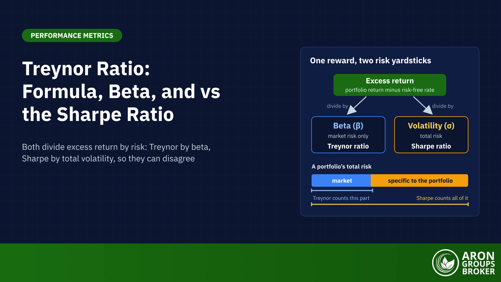

The Treynor ratio is a risk-adjusted return measure that divides excess return by beta. Excess return is the portfolio’s return minus the risk-free rate. Beta measures a portfolio’s sensitivity to overall market movements, so a higher Treynor ratio means more excess return per unit of market risk.
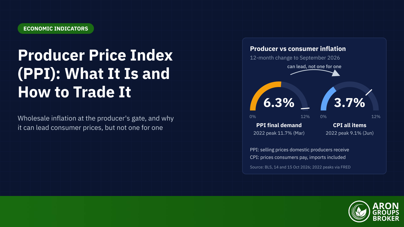
The hurdle in the numerator has risen. Three-month Treasury bills averaged 0.04% across 2021 and 3.94% in September 2026, on Federal Reserve data (discount basis). On 28 October 2026 the Fed held its target range at 3.75% to 4.00%. That day the 13-week Treasury bill yielded 4.11% on the US Treasury’s coupon-equivalent basis. At October 2026 rates, the same portfolio return buys far less excess return than it did in 2021.
This guide works through the Treynor ratio formula, then compares it with the Sharpe ratio on 50 years of US data. It shows where beta breaks down, then covers Jensen’s alpha, the information ratio, leverage and the measure’s honest limits.
- The Treynor ratio divides excess return over the risk-free rate by beta. It prices market risk, not total risk.
- In an illustrative example, an 8% return with a beta of 1.2 scores 3.24 against the 4.11% bill yield of 28 October 2026.
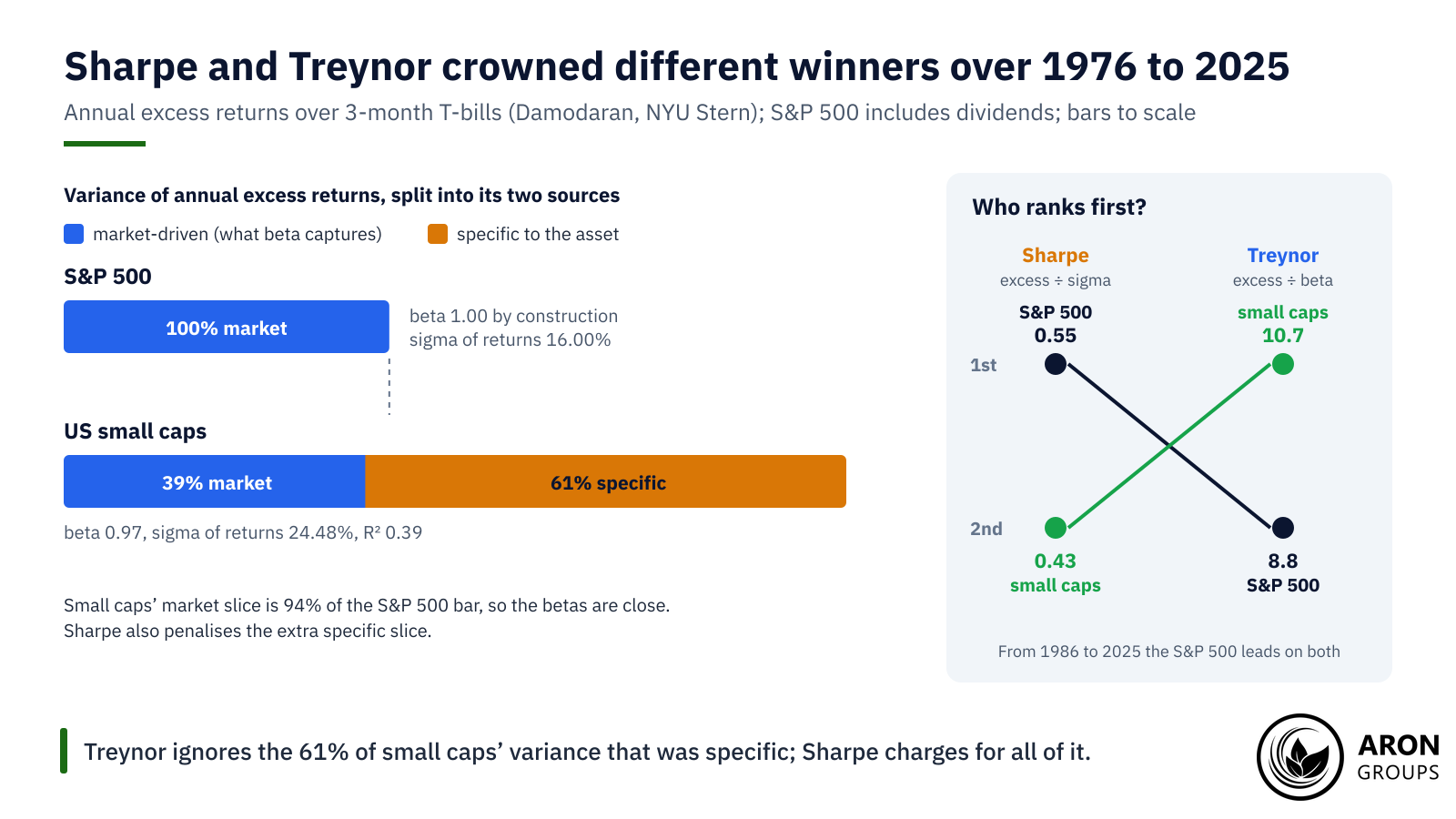
- From 1976 to 2025, US small caps beat the S&P 500 on Treynor, 10.7 to 8.8, but trailed on Sharpe, 0.43 to 0.55.
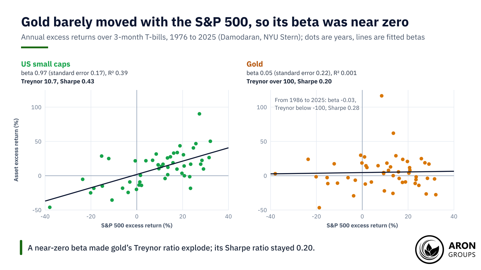
- Gold’s beta to the S&P 500 was 0.05 over the same years, which pushed its Treynor ratio above 100 and made it meaningless.
- With borrowing at the risk-free rate, leverage leaves the Treynor ratio unchanged in theory. Dearer financing, spreads and fees lower it.
What Is the Treynor Ratio?
The Treynor ratio, also called the Treynor measure or, in some texts, the reward-to-volatility ratio, ranks portfolios by excess return per unit of beta. It prices only systematic risk, not total risk: the market-wide part that diversification cannot remove. A higher ratio means the portfolio was paid more for each unit of market exposure.
Risk Disclosure
Trading forex and CFDs carries a high level of risk and can result in the loss of all your capital. This content is educational and is not investment advice. Never risk money you cannot afford to lose.
Treynor Ratio Definition and Origin
Jack Treynor set out the idea in “How to Rate Management of Investment Funds”, published in the Harvard Business Review in January/February 1965. A 2011 CFA Institute paper by Deborah Kidd says Treynor developed his index to measure reward to volatility, later misinterpreted as beta. The standard modern formula divides by beta, not by the standard deviation traders usually call volatility.
William Sharpe’s “Mutual Fund Performance” (Journal of Business, January 1966) built on Treynor’s work with the reward-to-variability ratio, now the Sharpe ratio. In “The Sharpe Ratio” (Journal of Portfolio Management, 1994), Sharpe described Treynor’s measure as an “average excess return to beta ratio”. Michael Jensen’s 1968 Journal of Finance paper on mutual funds from 1945 to 1964 added alpha.
Beta: The Market Risk in the Denominator
Beta is the covariance of a portfolio’s returns with a benchmark’s, divided by the benchmark’s variance. A beta of 1 means the portfolio moved one for one with the benchmark on average. A beta of 1.5 means about 1.5% for each 1% market move, and a negative beta means moving against it.
Beta measures market sensitivity, not total volatility. From 1976 to 2025, US small caps had a beta of 0.97 against the S&P 500. Yet their standard deviation was 24.48%, against 16.00% for the index. Gold, with a beta of 0.05, had a standard deviation of 24.68%. The S&P 500’s beta is 1 by construction when it is the benchmark. Against another index, period or return frequency, the estimate can differ.
In the capital asset pricing model (CAPM), beta sets the required return: the risk-free rate plus beta times the market’s excess return. Plotted against beta, that is the security market line. Multi-factor models add drivers such as size and value to the market factor. R-squared shows how much of a portfolio’s variance the benchmark explains; Kidd notes that a higher R-squared can lend more weight to beta.
The Treynor Ratio Formula
The Treynor ratio formula, also called the Treynor measure formula, is T = (Rp − Rf) / βp. Rp is the portfolio’s average return, and Rf the risk-free rate over the same period, often a Treasury bill yield. The beta, βp, is measured against a chosen benchmark. Because beta has no units, the result is in percentage points of excess return per unit of beta. All inputs need one basis, such as annual returns with an annual risk-free rate.
Mini Example: Scoring a Portfolio Against the Market
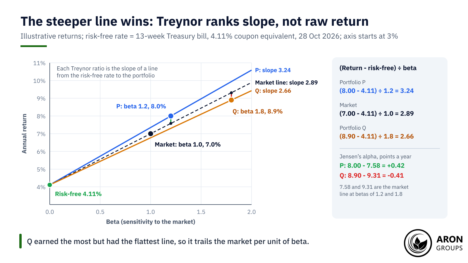
These numbers are illustrative, except the risk-free rate: the 13-week bill’s 4.11% on 28 October 2026. Portfolio P returns 8.0% with a beta of 1.2, and the market returns 7.0%. P’s Treynor ratio is (8.00 − 4.11) / 1.2 = 3.89 / 1.2 = 3.24.
The market’s ratio is (7.00 − 4.11) / 1.0 = 2.89, so P earns 0.35 points more per unit of beta. Jensen’s alpha gives the same verdict in points a year: 8.00 − (4.11 + 1.2 × 2.89) = 8.00 − 7.58 = 0.42.
With a 2.5% risk-free rate instead, P scores (8.0 − 2.5) / 1.2 = 4.58, or 4.6 to one decimal. Ratios computed with different risk-free rates are not comparable.
Reading the Result: The Market Sets the Bar
The market’s own Treynor ratio equals its excess return, because its beta is 1. That makes it the natural bar. With a positive beta, a portfolio beats the market’s ratio exactly when its Jensen’s alpha is positive. The link is alpha = beta × (Tp − Tm): an identity, not evidence of skill.
Illustrative portfolio Q in the chart returns 8.9% with a beta of 1.8. It earns more than P, yet scores (8.90 − 4.11) / 1.8 = 2.66, below the market’s 2.89. Its alpha is 8.90 − (4.11 + 1.8 × 2.89) = -0.41 points: the extra return did not pay for the extra beta.
Treynor Ratio vs Sharpe Ratio
The two measures share a numerator and differ in the denominator. The Sharpe ratio uses standard deviation while the Treynor ratio uses beta. Standard deviation counts total risk: market-driven swings plus risk specific to the portfolio. Beta counts the market part, so the choice turns on whether specific risk is borne.
| Feature | Treynor ratio | Sharpe ratio |
|---|---|---|
| Formula | (Rp - Rf) / βp | (Rp - Rf) / σp |
| Risk in the denominator | Beta: systematic (market) risk | Standard deviation: total risk |
| Needs a benchmark | Yes, to estimate beta | No |
| Suits | Well-diversified portfolios and parts of a diversified book | Standalone or undiversified portfolios; comparisons across asset classes |
| Unit | Points of excess return per unit of beta | Points of excess return per point of volatility |
| First published | Treynor, Harvard Business Review, 1965 | Sharpe, Journal of Business, 1966 |
| Weak spot | Beta near zero, negative or poorly estimated; negative excess return | Negative excess return, when more volatility looks better |
| US small caps vs S&P 500, 1976 to 2025 | 10.7 vs 8.8: small caps first | 0.43 vs 0.55: S&P 500 first |
Treynor ratio vs Sharpe ratio: one numerator, two risk yardsticks and, on 1976 to 2025 data, two different winners.
The Same 50 Years, Two Different Winners
Aswath Damodaran’s NYU Stern dataset, updated on 5 January 2026, gives annual US returns. From 1976 to 2025 the S&P 500, with dividends, averaged 13.17% a year (arithmetic mean). Three-month T-bills, taken as each year’s average rate, averaged 4.37%. That leaves an excess return of 8.80 points. Annual returns had a standard deviation of 16.00%, the Sharpe denominator used here. Betas here come from regressing annual excess returns on the S&P 500’s.
US small caps, the bottom size decile in Damodaran’s data, averaged 14.79%: an excess return of 10.42 points. His page does not say whether this series includes dividends. Their beta was 0.97, but their standard deviation was 24.48%. The Sharpe ratio ranks the S&P 500 first, 0.55 to 0.43. The Treynor ratio ranks small caps first, 10.7 to 8.8.
The gap is specific risk. Market moves explained 39% of small caps’ variance, an R-squared of 0.39; the other 61% was not explained by the S&P 500. Treynor ignores that 61%, while Sharpe charges for it.
When to Use the Treynor Ratio or the Sharpe Ratio
The practical rule follows from the denominators. The Treynor ratio suits well-diversified portfolios, where diversification has removed most specific risk, and single components of a larger diversified book. The Sharpe ratio suits standalone or undiversified funds and comparisons across asset classes, where total volatility is the risk actually borne.
Kidd makes the same point: because the Treynor ratio misses idiosyncratic risk, it is most relevant for a diversified portfolio. If small caps were a trader’s whole portfolio, the Sharpe verdict would apply. As one sleeve of a broad book, the Treynor verdict would carry more weight.
Q: Can a portfolio score well on Treynor but poorly on Sharpe?
A: Yes. US small caps did from 1976 to 2025, with a beta of 0.97. But 61% of their variance was not explained by the S&P 500, which Sharpe counts and Treynor ignores.
Where Beta Breaks: Gold, Low R-Squared and Negative Ratios
The Treynor ratio relies on a reliable beta and breaks with negative beta. Gold shows how. From 1976 to 2025 its beta to the S&P 500 was 0.05, with an R-squared of 0.001. Market moves explained almost none of its swings, and a standard error of 0.22 left the beta indistinguishable from zero.
Dividing gold’s 5.01-point excess return by 0.05 gives a Treynor ratio above 100, against 8.8 for the S&P 500. From 1986 to 2025 the beta turns slightly negative, at -0.03, pushing the ratio below -100. Gold’s Sharpe ratio stayed ordinary: 0.20 for 1976 to 2025 and 0.28 from 1986.
Negative Treynor Ratios Have Two Causes
A negative ratio can come from a negative excess return or from a negative beta, and the two mean opposite things. Take two illustrative portfolios that both trail the risk-free rate by 2 points. With a beta of 0.5 the ratio is -4.0; with a beta of 2.0 it is -1.0, so the riskier portfolio ranks higher.
A negative beta with a positive excess return is the reverse case. Under the CAPM, with a positive market premium, such an asset is expected to earn less than the risk-free rate. Beating that rate is therefore a strong result. Gold from 1986 is a real example: a negative ratio despite an alpha of 5.1 points a year. Its beta of -0.03 was indistinguishable from zero. Rankings mean most when both excess return and beta are clearly positive.
Jensen’s Alpha, the Information Ratio and the Wider Family
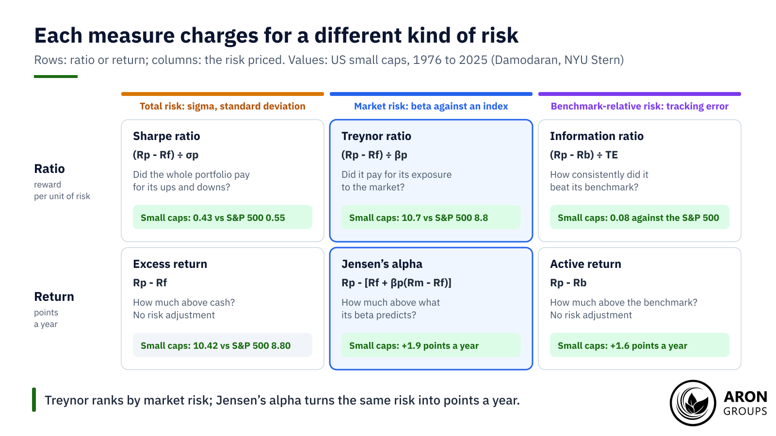
Performance measures differ in the risk they charge for. They also differ in form: a ratio that ranks, or a return in points a year. The Treynor ratio sits beside three close relatives.
Jensen’s Alpha
Jensen’s alpha is the return above what the CAPM predicts for a portfolio’s beta. In symbols, αp = Rp − [Rf + βp × (Rm − Rf)]. It is an absolute measure in points a year, often read as skill, while Treynor is a relative ranking measure. For US small caps from 1976 to 2025, alpha was about 1.9 points a year. Its standard error of 3.2 points left it indistinguishable from zero.
The Information Ratio
The information ratio divides active return, the portfolio’s return minus its benchmark’s, by tracking error, the standard deviation of that difference. A 2003 BIS report on asset management notes that specialist mandates often set targets as information ratios, relative return per unit of tracking error. Small caps’ mean return beat the S&P 500’s by 1.6 points a year, with a tracking error of 19.3 points: a ratio of 0.08. Compounded, the gap was 0.2 points a year.
Drawdown-Based Measures
Other measures change the yardstick again. The Sortino ratio counts only downside volatility, and the Calmar ratio divides return by maximum drawdown. A trader’s equity curve shows both kinds of risk, which a beta-based ratio cannot see.
Leverage, Costs and the Treynor Ratio
In theory, leverage does not change the Treynor ratio. If a trader borrows and lends at the risk-free rate, doubling exposure doubles both the excess return and beta. Their ratio stays the same, and so does the Sharpe ratio, since standard deviation also doubles.
Take an illustrative portfolio returning 8% with a beta of 1.2 and a standard deviation of 18%, against a 4% risk-free rate. Its Treynor ratio is 4 / 1.2 = 3.33 and its Sharpe ratio 4 / 18 = 0.22. Doubled with money borrowed at 4%, it returns 16 − 4 = 12%, so (12 − 4) / 2.4 = 3.33 again.
With borrowing at 6% instead, the return falls to 16 − 6 = 10%. The Treynor ratio drops to 6 / 2.4 = 2.50 and the Sharpe ratio to 6 / 36 = 0.17. Spreads, commissions and fees work the same way, and leverage magnifies losses as well as gains.
A CFTC customer advisory on forex warns that high leverage “amplifies both gains and losses”. It also says most OTC forex customers lose money once all credits, financing charges, fees and other costs are counted.
Key Point
Leverage rescales excess return and beta together. In the model above, financing above the risk-free rate, spreads and fees lower the ratio.

The Honest Limits of the Treynor Ratio
The Treynor ratio ignores unsystematic risk. That suits a sleeve of a diversified book but misleads for a concentrated account, where specific risk is borne in full.
It relies on CAPM assumptions and on a stable, backward-looking beta. Small caps’ beta was 1.01 for 1986 to 2025 and 0.89 for 2016 to 2025. Gold’s ranged from -0.03 to 0.31 across the three windows. Even over 50 years, small caps’ beta had a standard error of 0.17.
Rankings depend on the period. From 1986 to 2025 the S&P 500 led small caps on both measures: Treynor 9.5 to 8.7 and Sharpe 0.57 to 0.35. From 2016 to 2025 it led 13.5 to 7.8 and 0.87 to 0.40.
Benchmark choice and sample design matter too. An SEC investor bulletin on performance claims says that “it is important to compare apples to apples” when picking a benchmark. It also warns that past performance cannot predict future results and that back-tested performance is hypothetical. Out-of-sample testing helps, but a short sample still gives a noisy beta.
Where Aron Groups Fits
Aron Groups offers index CFDs such as SPXUSD, NDXUSD and DJIUSD, plus forex pairs and gold, on MetaTrader 5. For a trader, the Treynor ratio is a way to judge a strategy against an index. The platform’s trading report, opened from the History tab, summarises an account with figures such as drawdown and profit factor.
Monthly results logged in a trading journal can be set against an index’s monthly returns to estimate a strategy’s beta and Treynor ratio. Leverage on CFDs magnifies losses as well as gains, and past ratios do not predict future ones. A demo account with virtual funds, or a Nano account, lets traders test the arithmetic at small size. Neither removes the risk of loss in live trading.
Conclusion
The Treynor ratio asks how much excess return a portfolio earned per unit of market risk. It answers well for diversified portfolios with a stable, clearly positive beta, judged against the market’s own ratio over the same period.
It answers badly for concentrated positions, assets with little link to the market such as gold, and short or unstable samples. Alongside the Sharpe ratio, Jensen’s alpha and drawdown, it shows how well a portfolio was paid for its market exposure.
Frequently Asked Questions
Short answers to common questions about the Treynor ratio.
What Is a Good Treynor Ratio?
There is no universal threshold, because the ratio depends on the period, the benchmark and the risk-free rate. A positive ratio above the benchmark’s own, which equals its excess return, is the usual bar. From 1976 to 2025 that bar was 8.8 for the S&P 500.
Sharpe Ratio vs Treynor Ratio: Which Is Better?
Neither in general. The Sharpe ratio fits a whole or undiversified portfolio, because it counts total risk. The Treynor ratio fits a diversified portfolio or one part of a larger book, where market risk dominates.
What Is Treynor Ratio Analysis Used For?
Treynor ratio analysis ranks diversified portfolios, managers or strategy sleeves by reward per unit of market risk. Traders can apply it to their own results against an index, provided the beta estimate is reliable.
Can the Treynor Ratio Be Negative?
Yes. It is negative when excess return and beta have opposite signs, and those two cases mean different things. Gold from 1986 to 2025 had a positive excess return but a beta of -0.03, so its ratio fell below -100.