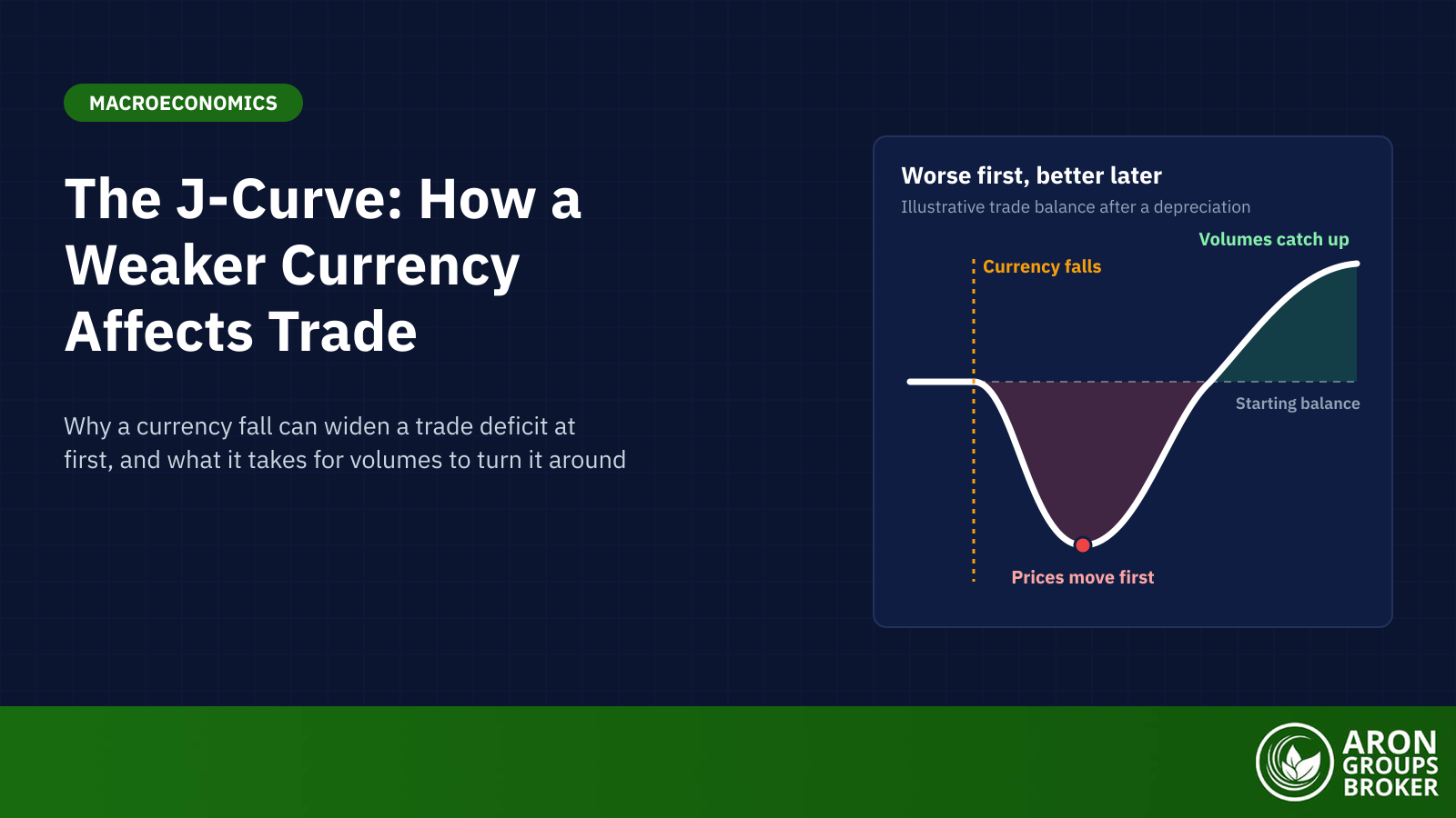

The J-curve, or J curve effect in economics, describes how a country’s trade balance can move after its currency depreciates or is devalued. The trade balance first worsens and then improves, tracing a J shape over time. Import and export prices react quickly, while volumes take longer to adjust. It is a tendency, not a law.
Japan’s 2026 trade data show why the idea matters. In September USD/JPY averaged 156.42, so a dollar bought 5.8% more yen than a year earlier (Federal Reserve). Yet Japan’s trade deficit that month was ¥536.6 billion, up from ¥277.7 billion in September 2025 (Ministry of Finance, provisional, 21 October 2026). Oil prices and chip exports moved those figures too, so the yen is only part of the story.
This guide explains why the balance dips, why it recovers and when it does not. It works through an illustrative example, the Marshall-Lerner condition, the US after 1985 and the research. It ends with how the idea differs from the private equity J-curve and a trading equity curve.
- The J-curve is the path a trade balance can follow after a depreciation: worse at first, better later.
- The dip comes from prices moving before volumes, while old contracts and habits hold quantities in place.
- Recovery needs large enough volume responses; in textbook terms, the Marshall-Lerner condition must hold.
- The dollar's monthly index peaked in March 1985, but the US deficit kept widening until mid-1987 before it narrowed.
- Evidence is mixed: Rose and Yellen found no reliable J in US data, and dollar invoicing changes the mechanics.
What Is the J-Curve?
The J-curve shows how a trade balance moves after a currency depreciation. A simple J curve definition: the balance first worsens in value terms, then improves beyond its starting point. Depreciation means the currency buys less foreign currency than before; a devaluation is the same move when a government lowers a fixed rate. The trade balance is exports minus imports of goods and services, part of the current account in the balance of payments.
Risk Disclosure
Trading forex and CFDs carries a high level of risk and can result in the loss of all your capital. This content is educational and is not investment advice. Never risk money you cannot afford to lose.
Where the Term Comes From
Stephen Magee’s 1973 paper in the Brookings Papers on Economic Activity is the usual citation for the J-curve. It studied the dollar’s 1971 devaluation. The US trade balance went from a $2.2 billion surplus in 1970 to deficits of $2.7 billion in 1971 and $6.8 billion in 1972. Magee called the J-curve “widely discussed”, so the term was already in use. He quoted The Wall Street Journal of 18 December 1972, which said the effect “can be plotted in what economists call a J-curve”.
Reading a J Curve Graph
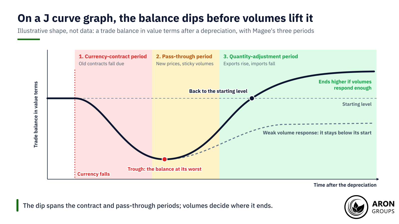
A J curve graph puts time on the horizontal axis and the trade balance in value terms on the vertical one. The curve falls after the depreciation, bottoms out, then climbs as volumes respond. Magee split this short run into three parts: the currency-contract period, the pass-through period and the quantity-adjustment period.
Why the Trade Balance Dips First
Right after a depreciation, trade volumes cannot adjust instantly. Goods ordered earlier are still arriving, and buyers need time to switch suppliers. Prices adjust first, so imports cost more and exports earn less, at least in the textbook case. In value terms the trade balance deteriorates in the short run.
The Currency-Contract and Pass-Through Periods
In Magee’s terms, the currency-contract period is the brief spell “in which contracts negotiated prior to the change fall due”. The currency of those contracts decides what happens. In the textbook case, exports are priced in the exporter’s currency and imports in foreign currency. The import bill then jumps in local money, while export receipts are worth less abroad. In the pass-through period, new contracts carry new prices, but quantities have barely moved. Dearer imports can also add to inflation.
The Invoicing Caveat: Dominant Currency Pricing
The textbook case is far from universal. About 40% of global exports are invoiced in US dollars, well above the share sold to the United States (ECB, June 2025). Under dominant currency pricing, exporters set prices in dollars and adjust them slowly. A depreciating country’s exporters then earn the same dollars, worth more at home, and foreign buyers see no discount.
A BIS working paper by Casas, Díez, Gopinath and Gourinchas makes the point. The real consequences of exchange rate swings, it says, “depend critically on how firms set prices in international markets”. Gopinath and co-authors (2020, American Economic Review) found the dollar exchange rate “quantitatively dominates the bilateral exchange rate” in price and volume estimates. A 1% dollar appreciation predicted a 0.6% fall in trade volumes between other countries within a year.
Why the Balance Recovers
Over time cheaper exports rise and pricier imports fall. Foreign buyers switch towards the cheaper goods, while firms and households at home cut back on dearer imports. If those shifts are large enough, the trade balance then improves beyond its starting point. In IMF estimates for 60 economies, much of the adjustment came in the first year, though the full effect took several years.
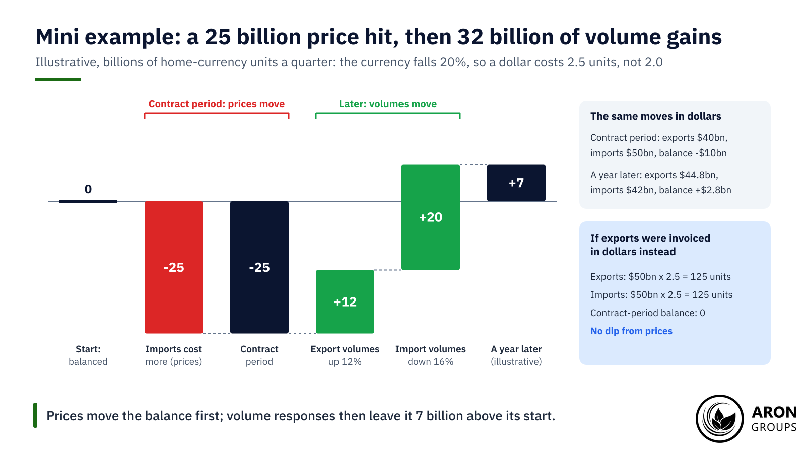
Mini Example: A 20% Fall in an Illustrative Currency
Take an illustrative economy whose exports earn 100 billion units of its currency a quarter, priced in that currency. It imports $50 billion of goods priced in dollars. At 2.0 units per dollar, imports also cost 100 billion units, so trade is balanced.
The currency then falls 20%, from $0.50 to $0.40, so a dollar costs 2.5 units. In the contract period, old prices and volumes stay put. Imports now cost 125 billion units, so the balance swings to a deficit of 25 billion. In dollars, exports earn $40 billion against $50 billion of imports, a $10 billion deficit.
Suppose that a year later export volumes are 12% higher and import volumes 16% lower. Exports bring in 112 billion units. Imports fall to $42 billion, or 105 billion units. The balance is now a surplus of 7 billion units, or $2.8 billion: worse first, better later.
Had the exports been invoiced in dollars, they would have earned 125 billion units at once, and the contract-period dip would vanish.
The Marshall-Lerner Condition
The recovery is not automatic. In the textbook model, the Marshall-Lerner condition must hold for the balance to improve. It says the sum of export and import demand elasticities must exceed one, in absolute value. A price elasticity of demand measures how far volumes move when prices change.
The standard derivation assumes trade starts roughly balanced, supply can expand without raising prices, and exchange rate changes pass through fully. It is a long-run condition. The J-curve is the short-run path, and the condition decides whether that path ends above its start.
In the mini example, suppose volumes move only 4% each way. Exports earn 104 billion units and imports cost 120 billion, so the balance ends at a deficit of 16 billion. With such small responses, the elasticities sum to well under one.
Key Point
A J needs both a short-run dip from prices and a long-run recovery from volumes. Without enough volume response, the balance can stay worse.
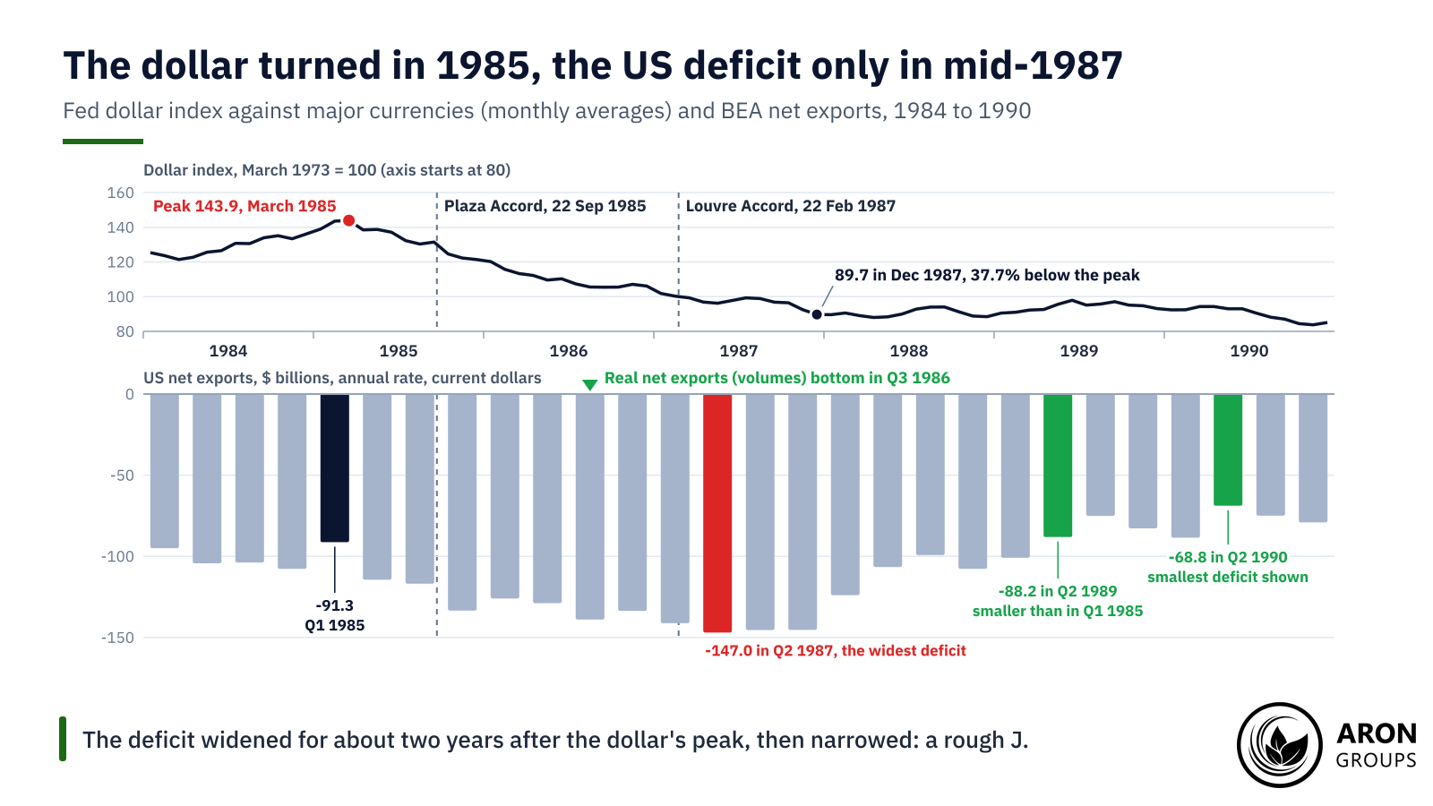
A Real J Curve Example: The Dollar After 1985
The swing of the US dollar in the 1980s is a much-cited J curve example. On the Federal Reserve’s index against major currencies, its monthly average peaked at 143.9 in March 1985 (March 1973 = 100). By August 1985, a month before the Plaza Accord, it was already 9.4% lower.
The accord’s G5 statement of 22 September 1985 said “some further orderly appreciation of the main non-dollar currencies against the dollar is desirable”. In Paris on 22 February 1987, the Louvre Accord aimed to “foster stability of exchange rates around current levels”. By December 1987 the index was 89.7, 37.7% below its peak.
The trade deficit did not shrink at first. BEA’s national accounts put it at $91.3 billion in the first quarter of 1985, at a seasonally adjusted annual rate in current dollars. It widened, with ups and downs, to $147.0 billion in the second quarter of 1987. It stayed near $145 billion for the rest of 1987, then narrowed to $99.3 billion by the third quarter of 1988.
By the second quarter of 1989, at $88.2 billion, the deficit was smaller than when the dollar peaked. Volumes had turned earlier: real net exports, in chained 2017 dollars, bottomed in the third quarter of 1986. That was three quarters before the nominal deficit peaked. Meanwhile US import prices rose 13.2% from March 1985 to December 1987 (BLS), even though oil got cheaper.
The data fit a J, but they cannot isolate the dollar’s role. Oil fell from $30.81 a barrel in November 1985 to $11.58 in July 1986 (WTI spot, Dow Jones via FRED). Growth at home and abroad also drives trade.
Britain After 1967
Sterling’s devaluation of 18 November 1967, from $2.80 to $2.40, is the other classic case. On OECD data in US dollars, Britain’s goods deficit was $1.69 billion in 1968, slightly wider than the $1.65 billion of 1967. In sterling terms the 1968 widening was larger. It shrank to $0.51 billion in 1969 and $0.04 billion in 1970, and 1971 brought a $0.50 billion surplus. Many other things changed too, so the pattern is suggestive rather than proof.
What the Evidence Says
Empirical support is mixed. Bahmani-Oskooee and Ratha’s 2004 survey in Applied Economics called the results “at best ambiguous”. Rose and Yellen (1989) found no statistically significant J in aggregate US trade or in its trade with the other G7 countries.
Finer data give a patchier picture. In US trade with 18 partners, Bahmani-Oskooee and Ratha (2004) found no short-run J. In the long run, though, a real depreciation of the dollar improved the balance in most cases. Across 108 industries in Australia’s trade with the US, Bahmani-Oskooee and Wang (2007) found short-run effects in 64 and long-run gains in 35.
Backus, Kehoe and Kydland (1994) found trade balances negatively correlated with current and future terms of trade, but positively with past ones. Their terms of trade are import prices over export prices. Their working paper called the pattern an S-curve. In the IMF’s estimates, a 10% real depreciation came with a 1.5% of GDP rise in real net exports on average, with wide variation.
| Study | Data | Finding |
|---|---|---|
| Magee (1973), Brookings Papers | US after the 1971 devaluation | Contract currencies and pass-through shape the short run; a dip is "by no means inevitable theoretically" |
| Rose and Yellen (1989), Journal of Monetary Economics | US aggregate trade and bilateral trade with the G7 | No statistically significant J-curve |
| Backus, Kehoe and Kydland (1994), American Economic Review | International data | Negative correlation with current and future terms of trade (import over export prices), positive with past ones (the working paper's "S-curve") |
| Bahmani-Oskooee and Ratha (2004), Applied Economics | Survey of the literature | Results "at best ambiguous" |
| Bahmani-Oskooee and Ratha (2004), Journal of Economics and Finance | US bilateral trade, 18 partners | No short-run J; long-run improvement in most cases |
| Bahmani-Oskooee and Wang (2007), Australian Economic Papers | Australia's trade with the US, 108 industries | Short-run effects in 64; long-run gains in 35 |
| IMF World Economic Outlook (October 2015) | 60 economies, from the 1980s to 2014 | 10% real depreciation: real net exports up 1.5% of GDP on average |
| Gopinath and co-authors (2020), American Economic Review | Over 2,500 country pairs | The dollar rate dominates bilateral rates in pass-through and trade volumes |
Selected J-curve evidence, from the papers and reports named in the text.
The Asian Crisis Does Not Fit the Textbook
The 1997 to 1998 Asian crisis is sometimes cited as a J-curve case, but it fits poorly. Thailand’s current account moved from a deficit of 2.0% of GDP in 1997 to a surplus of 12.8% in 1998. South Korea’s went from a deficit of 1.7% to a surplus of 12.5% (RBA, from IMF and CEIC data). The Reserve Bank of Australia traced much of the swing to “a sharp decline in imports” as domestic demand contracted. Exports showed “little change in volumes” at first.
Q: Does a weaker currency always shrink a trade deficit?
A: No. The result depends on how far volumes respond, which currency trade is priced in, and growth at home and abroad. Some episodes show no J at all.
Why the J-Curve Matters for FX Traders
For FX traders, the J-curve explains why a weaker currency does not instantly improve the trade balance, and may hurt it first. A widening deficit after a fall can be a lag rather than a failure. Trade is one input in how currency strength is determined, alongside interest rate differentials and risk appetite.
That shapes market narratives around currency moves, trade deficits and policy. Governments sometimes devalue, or push the rate down through currency intervention, hoping to fix a deficit. The J-curve warns that the deficit can worsen first and the fix can be slow.
Japan in 2026 shows how hard the effect is to read in real time. In September its imports rose 18.9% from a year earlier and exports 16.7%, with semiconductor exports up 49.4% (Ministry of Finance, provisional). Crude oil imports rose 51.1% in value on 3.1% more volume, so most of the rise came from price.
Brent averaged $114.16 a barrel in September, 67.9% more than a year earlier (EIA). That dwarfs the dollar’s 5.8% rise against the yen over the same months. A J-curve would show up in volumes over several quarters, if at all. One month of data cannot separate it from oil prices and demand.
The J-Curve vs the Private Equity J-Curve and Your Equity Curve
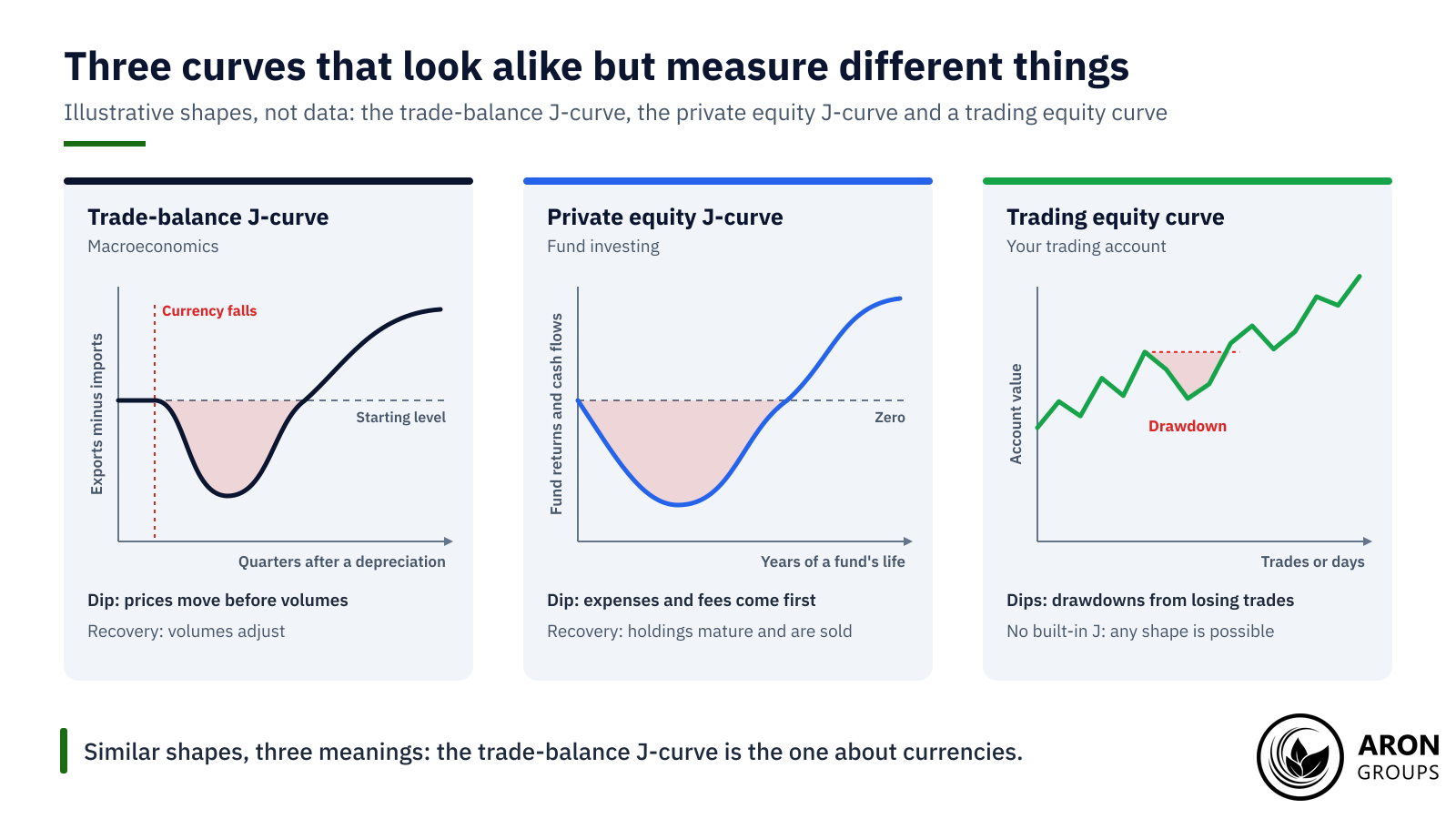
The trade-balance J-curve is an economics concept. The private equity J-curve describes fund returns that start negative. Returns and cash flows are negative in a fund’s early years, because expenses and fees come first and capital takes time to invest. Returns turn positive as holdings mature and are sold.
The J-curve is different from your trading equity curve, which plots your account’s value over time. Its dips are drawdowns from losing trades, not a built-in phase. A J shaped curve also appears in biology, where it describes a population growing exponentially before limits bite. Same shape, different domains.
The Honest Limits of the J-Curve
The J is a pattern, not a law. Magee wrote that the worse-before-better pattern, though it had some support, was “by no means inevitable theoretically”. Its timing also varies from case to case.
A trade balance also moves with growth, oil prices and demand, not only the exchange rate. The national accounts tie the current account to saving and investment, but that identity cannot show which moved first. Production abroad weakens the link as well. After the yen fell about 35% in real effective terms from late 2012, Japan’s real goods exports stayed broadly flat (IMF, 2015).
The IMF linked that to offshoring: overseas investment by Japanese subsidiaries was about 25% of manufacturing investment. For traders, a currency’s reaction to trade data is a tendency, not a rule. Positions can lose money whichever way the data surprise.
Where Aron Groups Fits
Aron Groups offers forex pairs that trade data can move, such as USD/JPY, EUR/USD and GBP/USD, on MetaTrader 5. The economic calendar lists scheduled releases such as inflation data and central bank decisions. Japan’s October trade figures are due on 18 November 2026. Currency reactions to such releases are tendencies, not rules. Leverage cuts both ways: a CFTC advisory warns that it “amplifies both gains and losses”.
Stop orders can limit losses, but an SEC investor bulletin warns that a triggered stop’s fill can deviate significantly from the stop price. A Nano account trades from 0.01 nano lots, and a demo account allows practice with virtual funds.
Conclusion
The J-curve explains why a weaker currency can hurt a trade balance before it helps. That is the core of J curve economics: the exchange rate moves at once, while volumes take quarters to respond.
The recovery needs volume responses large enough to meet the Marshall-Lerner condition, and the evidence for a clean J is mixed. Dollar invoicing, oil prices and growth often blur the pattern, and Japan’s 2026 data show the oil effect.
Frequently Asked Questions
Short answers to common questions about the J-curve.
What is the J curve in simple terms?
It is the path a trade balance can follow after a currency falls: worse at first, better later. Imports cost more before volumes respond, so the balance dips, then recovers if exports rise and imports fall enough.
How long does the J-curve last?
There is no fixed length. In IMF estimates, much of the adjustment comes in the first year. After the dollar’s 1985 peak, the US deficit kept widening for about two years.
What is the Marshall-Lerner condition?
It says a depreciation improves the trade balance if export and import demand elasticities sum to more than one, in absolute value. The textbook version assumes balanced trade at the start and supply that can expand.
Is the J curve in economics the same as the private equity J-curve?
No. The trade-balance J-curve tracks exports minus imports after a depreciation. The private equity version tracks a fund’s returns, which start negative because of fees and expenses and turn positive as investments are sold.